Expander operates on the following types of data:
a) Gene expression data û For most of EXPANDER's steps for analysis of gene expression data, the technique used for obtaining the expression estimates doesn't make a difference. Whatever technique (e.g., expression arrays, RNA-Seq) was used, the input expression data should be summarized in a matrix (tab-delimited txt file; see File Formats section) in which rows correspond to probes/genes and columns û to samples.
Values can be either relative intensities data,
expected as log 2 (R/G) values data (e.g. cDNA microarrays),
RNA-Seq counts OR absolute intensities data, expected
as positive expression levels (E.g. High-density oligonucleotide data).
Oligonucleotide data can be loaded with/without detection calls. Affymetrix
data can also be loaded from CEL files (If R is installed).
When analyzing RNA-Seq data, one way to obtain gene expression matrix is to use TopHat (http://tophat.cbcb.umd.edu/tutorial.html ) to align the sequenced reads to the relevant genome, and then use Cufflinks (http://cufflinks.cbcb.umd.edu/howitworks.html ) or HTSeq (http://www-huber.embl.de/users/anders/HTSeq/doc/count.html#count ) to obtain gene (or transcript) expression estimates from TopHat output.
If one wishes to perform functional analysis or promoter analysis, an ID conversion file should be loaded along with the data file. The conversion file maps each probe ID (first column) in the data file into a corresponding conventional gene ID that is used in the GO annotation and TF fingerprint files that are supplied with EXPANDER. The conversion file can be loaded in the middle of the session too, by Data >> Load Conversion File.
b) Similarity data û a pre-calculated similarity matrix
c) Gene group data û contains predefined groups of genes. In this data type, the conventional gene IDs that are used by EXPANDER in the GO annotation and TF fingerprint files are expected.
For details regarding the Gene ID convention that is used for each organism, refer to the Supplied Files section.
For details regarding the data files formats see the File Formats section.
d) Gene Ranking Analysis (GSEA) û contains predefined ranked genes. In this data type, the conventional gene Ids that are used by EXPANDER in the Gene Set Enrichment Analysis are expected.
For details regarding the data files formats see the File Formats section.
e) ChIP-Seq data û contains discovered peaks of Transcription Factor(TF) ChIP-Seq experiment in BED or GFF3 formats (see File Formats section).
Loading gene expression data:
To load tabular expression data, select: File >> New Session. From the submenu select Expression Data >> Tabular Data File.
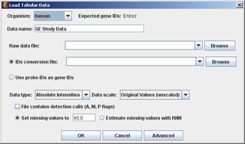
When selecting Tabular Data File, the following dialog box will appear:
Data type and scale are to be determined according to the input file. If the file contains missing values, these values will be estimated upon loading the data either by setting them to and arbitrary value (if the æSet missing value to ____Æ option is selected) or by utilizing the KNN (K-Nearest Neighbors) method (if the æEstimate missing values with KNNÆ option is selected). If the file contains Affymetrix detection calls data, the relevant check box must be checked. You may change / erase the default floor value, to which all entries that are below that value will be set (this option is available only for absolute intensities data).
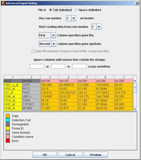
Advanced Input Dialog: Upon pressing the æAdvancedÆ button after filling the æRaw Data FileÆ field, an æAdvanced Input DialogÆ appears. This dialog box can be used in order to facilitate the data load of files that are not in the required format. The first few rows and columns of the data are displayed in a table, demonstrating the way the data is read by the program according to the current input values.
To load expression data from CEL files, select: File >> New Session. From the submenu select Expression Data >> CEL Files.
The load of CEL requires installation of R software (see R External Application section) along with specific packages, as detailed below. An open internet connection is also required for this operation.
Expander supports CEL files of three chip types:
1. 3' Gene Expression - requires Bioconductor ôaffyö package
2. Whole-Transcript Gene Expression (Gene 1.0 chips) û requires the prior installation of a cdf package for the used chip (see links below).
3. Alternative Splicing (Exon 1.0 chips) requires the prior installation of a cdf package for the used chip (see links below). * Please note that we estimate the overall expression for the transcript, not exon-by-exon. Therefore, this becomes 'gene data' rather than 'alternative splicing data'.
When selecting CEL Files, the following dialog box will appear:
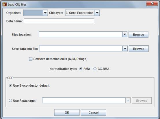
Please choose the relevant organism and chip type. Then browse to the folder where the CEL files are located (Files location), and choose where to save the expression file resulting from the CEL files preprocessing.
Preprocessing and normalization method: The default method in Expander is RMA. However, for 3' gene expression arrays, you may select GC-RMA instead (taking into account GC-content bias). Before using GC-RMA, please make sure you have the ôgcrmaö R package installed (see R External Application section).
CDF environment choice: You may use the default Bioconductor CDF environment for the chips or browse to an alternative CDF package which you have already installed in R. For whole transcript and alternative splicing chips (for which there is no default Bioconductor CDF environment), you will need to supply an alternative CDF package (see links below).
Note: GC-RMA requires the probe sequence information of the chip. If you decide not to use the default Bioconductor CDF environment, and have GC-RMA as the preprocessing method, you must have the suitable probe package installed in addition to the CDF alternative package.á
Link for downloading CDF environment packages (for 2nd option):
http://www.bioconductor.org/packages/release/data/annotation/
If Expander cannot find your R software, a window will appear, asking you to specify its location. Please browse to the location of your R software. In Windows, R.exe file is likely to be located in the 'bin' folder of R software. In Linux, you may type 'which R' in the command line to find R path. If you have a few versions of R installed, please make sure to point Expander to a version in which the Bioconductor ôaffyö package has been installed.
Once the CEL files preprocessing is done, a corresponding tabular data file is generated and a 'Load Study' dialog will appear, as in loading Tabular Data.
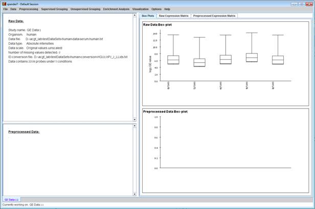
After loading a gene expression data set, a æSession DataÆ display tab is added to the main window (see example below). It contains information regarding the raw data file, a box plot chart, and an expression matrix visualization of the raw data. If detection calls exist in the data file, their statistics for each probe appear in 3 columns in the heat maps (expression matrices), in a scale between 0 and 1, corresponding to the relative part of each of the detection calls (P, M and A). The detection calls statistics for each condition are displayed in a separate tab in two tables (one for the raw data and another for the preprocessed data) and are presented in percent.
To start working on similarity data (no expression data associated) select File>>New Session>> Similarity Data...
The following dialog box will appear:
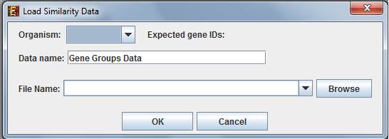
For details regarding the data files formats see the File Formats section.
After loading gene groups, a æSimilarity DataÆ display tab is added to the main window
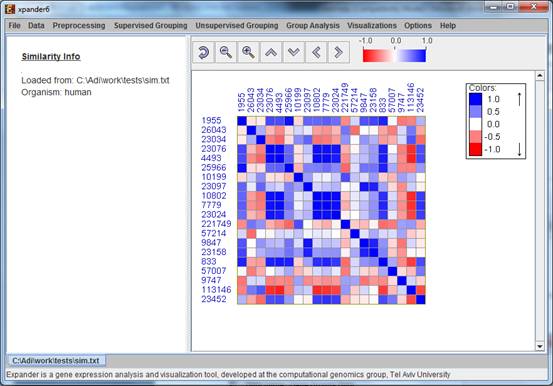
Currently similarity data can only be clustered using the Hierarchical clustering procedure by selecting Unsupervised Grouping>>Hierarchical Clustering>>Cluster... The resulting tree can be used to generate groups (for further details see Hierarchical Clustering).
To start working on gene groups (no expression data associated) select File>>New Session. From the submenu select Gene Groups.
The following dialog box will appear:
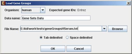
For details regarding the data files formats see the File Formats section.
After loading gene groups, a æSession DataÆ display tab is added to the main window (see example below). It contains information regarding the data file, and a table describing the different groups (serial number, name and size). Group names can be modified, by editing the corresponding cell in the table. Upon clicking on a row in the table, the corresponding group pane appears on the right. It contains a list of the genes in the group and a view of their chromosomal positions. If a network file has been loaded (via Data>>Load Network), the sub-graph, induced by the group is displayed as well.

To load ChIP-Seq data, select: File >> New Session. From the submenu select "ChIP-Seq Data".
The following dialog box will appear:
áááááá 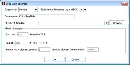
Select the organism and its reference genome that correspond to the ChIP-Seq experiment.
For details regarding the data BED/GFF3 files formats see the File Formats section.
Gene hit range:
This option allows choosing the gene range to be searched for peak hit.
The range is selected in the following way:
Start position upstream to the Transcript Start Site (TSS) and end position downstream to the TSS or to the Transcript Termination Site (TTS).
Note that the start position is a non-positive value.
There is an option to select more than 1 closest gene to peak by changing "Selecting top k closest genes" field and to set a distance bound for k>1 closest gene to peak.
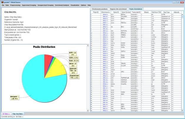
After loading a ChIP-Seq data, a æChIP-Seq Study DataÆ display tab is added to the main window (see example below). It contains information regarding the raw data file, a pie chart, a chromosome visualization of the mapped genes positions, a region hits enrichment bar chart, and a peaks annotations table. The pie chart contains the peaks distribution of the first closest gene hits. Each peak was mapped to the closest gene with regard to the TSS and mapped to one of the following regions: Upstream of the TSS, 5UTR, Exon, Intron, 3UTR, Downstream of the TTS or Intergenic (i.e., regions between genes). Chromosome visualization displays mapped genes to peaks with option to show or not to show the gene's strands. Region hits enrichments displays the enrichment test using binomial p-value was performed in order to evaluate the randomness of peaks falling in a specific region (excluding "Intergenic" region), for example, it can be seen that under 5UTR bar, peaks fall by random in this region with p-value 3.87E-133. This option is currently available only for human and mouse datasets.

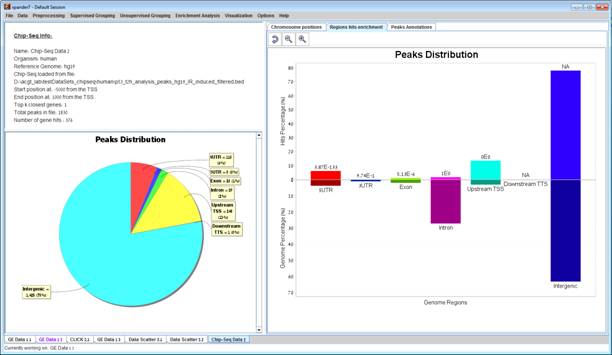
The peaks annotation table (see below) displays details for each peak û Peak ID (row number in ChIP-Seq file), Chromosome Position of the peak with a link to UCSC genome browser, Gene ID of the mapped gene to peak (blank if the peak was not mapped to a gene), Gene symbol, UCSC Transcript ID, Strand, Distance from TSS (negative/positive for upstream/downstream), Sequence type for the peak's mapped region and Intensity" or "Q-value" depending on the uploaded file format (BED or GFF3).
Pie chart, chromosome visualization and Region hits enrichment bar chart can be increased or decreased using the mouse scroll wheel.
Fetch ChIP-Seq peaks sequences
To fetch FASTA sequences for the peaks select Data->Fetch ChIP-Seq Sequences...
The following dialog box will appear:
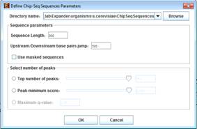
Select the directory path where the created files will be inserted (Default folder is á
<path to>/Expander/organisms/<Selected organism>/ChipSeqSequences/).
Sequence parameters:
Please see image demonstration below.
À Sequence Length (Default is 300 bps) - áin base pairs
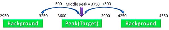
À Upstream/Downstream base pairs jump (Default is 500 bps) û For each peak, two background sequences of length 300 bps are created 500 bps upstream and downstream from the middle position of the peak.
À Use masked sequences û Fetch sequences from repetitive masked FASTA genome.
Select number of peaks:
À Top number of peaks û top peaks are selected by their score (Intensity or q-value). If the no score was added then the peaks are selected according to their row line position in the file.
À Peak minimum score û available only in BED format. Peaks are selected if their score is above the selected minimum score.
À Maximum q-value û available only in GFF3 format. Peaks are selected if their q-value is below the selected maximum q-value.
After clicking OK, 3 files will be created in the selected folder:
À sequences.fa û contains the FASTA sequences of the selected peaks and their two background sequences.
À target.txt û contains identifiers of the selected peaks.
À background.txt û contains identifiers of the selected peaks and their background identifiers.
Notes
Fetching non-masked sequences process should take on average ~1-2 seconds for about ~5000 sequences of length 300 bps.
Fetching masked sequences might take longer time û on average ~10 seconds for ~5000 sequences of length 300 bps.
The created files can be used as input data in our AMADEUS motif finding software.