The following preprocessing operations can be performed using EXPANDER:
1) Flooring (Preprocessing >> Floor Data): setting all expression values that are below a certain threshold (set by the user) into that threshold. This can be done either by setting the floor value itself, or by setting the percentile that should be used as floor value.
2) Merging conditions (Preprocessing >> Merge conditions): merging a selected set of condition profiles (columns) in the dataset into one profile, in which each entry holds the average value of the merged entries.
3) Merging probes according to gene ID (Preprocessing >> Merge Probes by Gene ID): automatically shrinks the matrix so that all rows of probes from the same gene are merged into one average row, identified by the corresponding gene ID.
4) Normalization: required in order to remove systematic variation, i.e. variation arising from reasons other than biological differences between RNA samples. Expander performs normalization only for absolute intensities data, since it is assumed that the relative intensities data (e.g. cDNA microarrays) is already normalized, as it is input after performing log ratio (log2R/G).
Normalization can be performed using the following schemes:
a) Quantile normalization (Preprocessing >> Normalization >> Quantile), in which the whole data is used.
b) Non-linear baseline normalization (Preprocessing >> Normalization >> Non Linear Baseline), which uses a baseline array (can be selected by the user). In this scheme a normalization function is calculated using pseudo Loess regression of the M vs. A scatter plot. The subset of genes that are used to evaluate the normalization function can be set to ‘all genes’ (recommended when most genes in the dataset are expected to be constantly expressed) or a ‘rank invariant set’ of genes (recommended when there can be a large number of differentially expressed genes).
For more details regarding the normalization schemes see the References section.
5) Condition filtration: the conditions used in the analysis can be manually filtered by selecting: Preprocessing >> Filter Conditions. This will bring up a dialog box in which the user can select the required conditions from a list.
6) Gene (probe) filtration: can be performed in order to filter out some of the constantly expressed genes, and perform downstream analysis on a smaller informative subset of the genes.
Probe filtration can be performed using the following schemes:
a) t-Test (Preprocessing >> Filter Probes >> t-Test): When using this method, only probes that demonstrate differential expression between two condition subsets are selected.
b) SAM - Significance Analysis of Microarray (Preprocessing >> Filter Probes >> SAM): selects probes that demonstrate differential expression between conditions subsets. You may choose 2 or more subsets (multi-class tests are supported). This method uses permutations to get an ’empirical’ estimate for the FDR of the reported differential genes (for details see the References section). Before using SAM, please make sure you have R software along with the “samr” package installed (see R External Application section).
c) Fold Change (Preprocessing >> Filter Probes >> Fold Change): when using this method only genes that are over/under expressed by at least n fold in at least k arrays are selected (n and k are determined by the user). The fold change can be calculated in relation to (a) a selected baseline array (b) the minimal expression value of the gene OR (c) the reference value when working on relative intensities (depending on the user’s selection).
d) Variation (Preprocessing >> Filter Probes >> Variation): In this method, the k most variant genes are selected (k is determined by the user). Variance is used to measure variation for relative intensities data, and Coefficient of Variation is used to measure variation for absolute intensities data.
e) Detection calls (Preprocessing >> Filter Probes >> Detection calls): in this method probes/genes are filtered according to the number of expression signals for which the detection call is ‘P’ (Present). It can only be operated if the data file contains detection info.
f) Load Probe Subset (Preprocessing >> Filter Probes >> Load Probe Subset): the filtered set is loaded from an external txt file (for details regarding the format please see the File Formats section).
7) Divide by Base (Preprocessing >> Divide by Base) – Divides each entry in a profile (a column) by the corresponding entry in the profile of a selected base condition. This can be done for all conditions or for subsets of the conditions.
8) Log data (Preprocessing >> >> Log Data) – Performs log2 operation on each entry
9) Standardization: When expression values between different genes are very different, but general expression patterns are similar (high Pearson Correlation values), we would expect to see this similarity when looking on a pattern display. Since the absolute values of expression are different, a manipulation is required, in order to view the patterns on the same scale. This manipulation is called standardization.
Standardization can be performed using the following schemes:
a) Mean 0 and Variance 1 (Preprocessing >> Standardization >> Mean 0 and Variance 1) – normalizes each expression pattern to have a mean of 0 and a variance of 1. This method is appropriate in most cases when working on genes.
b) Fixed norm (Preprocessing >> Standardization >> Fixed Norm) - normalizes each expression pattern to have a fixed norm i.e. expression levels are divided by the norm of that expression vector (the root of sum of squares of that vector). This method is appropriate when different mean values or variances are expected for different patterns (e.g. when working on conditions and expecting larger variance in later phases of a response.
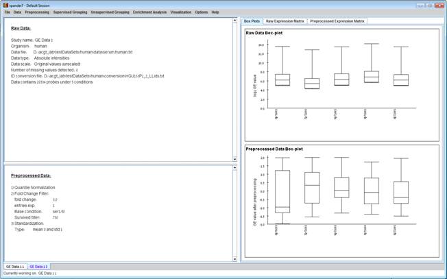
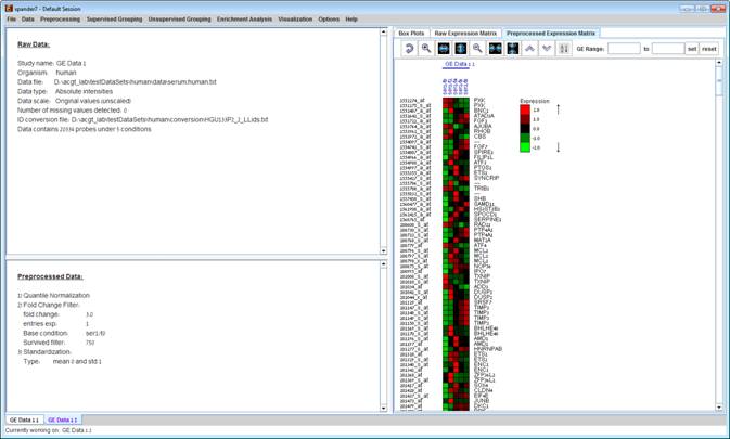
After performing a preprocessing operation, the information regarding the operation is added to the ‘Preprocessed Data’ section in the ‘Session Data’ tab. In addition, the ‘Preprocessed Data box plot’ and ‘Preprocessed Expression Matrix’ are automatically updated according to the new values in the data.
Upon selecting Preprocessing >> Undo the data is changed to be as it was before the most recent preprocessing operation was performed, and the corresponding information is removed from the ‘Preprocessed Data’ section. The ‘Preprocessed Data box plot’ and ‘Preprocessed Expression Matrix’ are automatically updated accordingly.
All the above operations can be performed before running further analysis on the data and generating displays. When attempting to perform further preprocessing operations after analysis results and visualizations have been generated, the following dialog box appears:
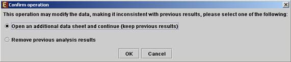
Upon choosing to open an additional data sheet, a new data set view tab called ‘Data Sheet 2’ is added to the main frame. The title of this tab is highlighted (colored in purple), indicating that it is now the active data sheet (i.e. all further operations refer to this data sheet). The active data sheet is automatically changed according to the selected (front) visualization tab.
Preprocessed gene expression data can be saved to a file at any time be selecting Preprocessing >> Save Preprocessed Data. The data is written in the same format defined for input GE data.