The goal of clustering is to partition the
genes into distinct sets such that genes that are assigned to the same
cluster should have similar expression patterns, while genes assigned to
different clusters should have non-similar expression patterns.
Usually there is no one solution that is the ‘true’ mathematical solution for
this problem, but a good clustering solution should have two merits:
(1) High homogeneity (average similarity between genes from the same cluster).
(2) High separation (average distance/dissimilarity between genes from different clusters).
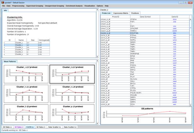
After operating one of the clustering algorithms a clustering results view appears. The view contains information about the solution and its quality including the method and parameters that were used to obtain it, number of clusters, number of singletons (probes that were not assigned to any cluster), overall homogeneity and separation, as well as the size and homogeneity of each cluster. This summary can be used to compare different solutions.
In order to apply a clustering algorithm to the data, select the required algorithm from the Unsupervised Grouping >> Clustering menu (options are: KMeans, CLICK, SOM). You can also use the agglomerative hierarchical clustering algorithm by extracting a partition from an existing hierarchical tree, by selecting Unsupervised Grouping >> Hierarchical Clustering>> Generate Groups (For details about building such a tree, please go to Hierarchical Clustering).
Currently similarity data can only be clustered using the Hierarchical clustering procedure by selecting Unsupervised Grouping>>Hierarchical Clustering>>Cluster... The resulting tree can be used to generate groups (for further details see Hierarchical Clustering).
An existing clustering solution can be loaded from a file by selecting Unsupervised Grouping >> Clustering >>Load Solution (For details regarding the clustering solution file format, refer to the File Formats section). The CLICK algorithm is not designed to find clusters under the size of 15 probes, so it might fail in clustering small datasets.
Fill the required input data in the algorithm
input dialog box and press the ‘Ok’ button.
The parameters required for each method are as follows:
|
Algorithm |
Required parameters |
|
KMeans |
Expected number of clusters. |
|
SOM |
Grid width, grid length (width*length >= number of clusters) and number of iterations. |
|
CLICK |
Homogeneity value (0-1): allows the user control over the homogeneity of the resulting clustering, i.e. the average similarity between elements in the same cluster. This parameter serves as a threshold in various steps in the algorithm, including the definition of cluster kernels, singleton adoptions and kernel merging. The default value for this parameter is the estimated homogeneity of the true clustering. The higher the value assigned to this parameter the tighter the resulting clusters. |
|
Hierarchical tree partition |
Distance threshold (if extracting by distance): 0-1 the minimal tree distance that is required for two nodes to be assigned to the same group · It is also possible to partition the tree according to manual node selection that is performed on the hierarchical view (see Hierarchical Clustering). |
Details about the algorithms can be obtained through the relevant articles in the References section.
After clustering is performed, a clustering solution visualization tab is added to the main window. It contains the following views:
Information regarding the clustering algorithm, number of clusters, number of un-clustered elements (singletons), and numerical measures of the clustering quality, including:
d) Overall average homogeneity - calculated as the average value of similarity between each element and the center of the cluster to which it has been assigned, weighted according to the size of the cluster.
e) Overall average separation – calculated as the average similarity between mean patterns of different clusters, weighted according to their sizes.
f) Clusters table - contains the number, name (label), size and homogeneity of each cluster. The name of a cluster can be changed by editing the corresponding cell in the table.
Mean Patterns of all clusters with error bars (±1 STD).
Upon selecting a cluster (from the clusters table or from the mean patterns view), the corresponding cluster pane is displayed on the right. It contains a list of probes, probe patterns, expression matrix (heat map) and the chromosomal locations of the genes. Similarity matrices for probes within the cluster as well as for conditions are also displayed in this tab, if the relevant options in the display settings are selected (see the Settings section). If a network file has been loaded (via Data>>Load Network), the sub-graph, induced by the cluster is also displayed in the cluster pane.
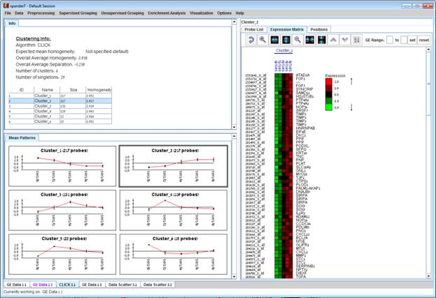
After performing enrichment analysis (for details see the Enrichment Analysis Tools), if enrichment has been detected in the selected cluster, the corresponding histogram and analysis information are added to the single cluster view.
In order to allow comparison between groups and patterns, the displayed expression patterns are automatically standardized to have mean = 0 and STD = 1.
A clustering solution can be saved using the File >> Export to text option (with the corresponding clustering view as the selected tab) OR by using the File>>Save All option, which will export all solutions within a session to text and image files. A clustering solution can be reloaded using the Unsupervised Grouping >> Clustering >> Load Solution.