Biclustering is clustering of both genes and conditions of the data into subgroups that are not necessarily disjoint. It enables the user to detect genes that are co-regulated in only a subgroup of the conditions, and does not force genes to belong exclusively to one cluster. It is useful when working on datasets which contain a large number of conditions.
Expander incorporates two Biclustering algorithms: ISA (Iterative Signature Algorithm) and SAMBA algorithm (for details see the References section). Before using ISA, please make sure you have R software along with the “eisa” package installed (see R External Application section).
In order to apply the ISA algorithm to the data select Unsupervised Grouping>>Bi-Clustering>>ISA. This operation does not require parameter input.
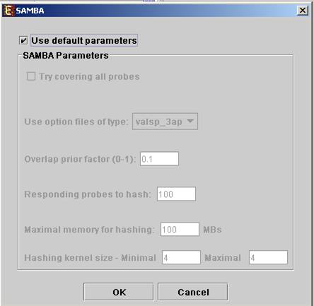
In order to apply the SAMBA algorithm to the data select Unsupervised Grouping>>Bi-Clustering>>SAMBA. The following dialog box will appear:
It enables the configuration of some of the parameters for the algorithm. The following table specifies the different parameters that can be set via this dialog box:
|
Field |
Description |
|||||||||||||||||||||||||||||||||||
|
Use default parameters |
When checked, biclustering parameters (described below) are set automatically (this option is recommended unless the user is familiar with the parameters). |
|||||||||||||||||||||||||||||||||||
|
Option files type |
The user can select one out of 6 options. The following table describes the advantages and disadvantages of each option:
We recommend the valsp_3ap option (set as default), since it is very flexible, and produces good results also for data that was not normalized properly or for non gene-expression data. |
|||||||||||||||||||||||||||||||||||
|
Always cover all genes |
When checked, the solution will cover each gene at least once (each gene will be included in one or more biclusters). |
|||||||||||||||||||||||||||||||||||
|
Always cover all conditions |
When checked, the solution will cover each condition at least once (each condition will be included in one or more biclusters). Un checking this option will cause a reduction in the number of biclusters, and the algorithm will run faster. |
|||||||||||||||||||||||||||||||||||
|
Overlap prior factor
|
Can take values between 0 and 1, describes extent of overlap that is permitted between two different biclusters in the same solution. The higher this parameter is, the more strict the algorithm will be regarding adding a new bicluster (will require less overlap between the new bicluster and the existing ones). |
|||||||||||||||||||||||||||||||||||
|
Number of responding genes to hash |
Can take values between 1 and the number of genes in the dataset. Default value is set to 100 (recommended unless data set size < 100). Has impact over the hashing stage in the algorithm. |
|||||||||||||||||||||||||||||||||||
|
Maximum hash size (in MB) |
Described the maximum memory size that can be used for the hashing part of the algorithm (the whole algorithm will take up about twice this size of memory). |
|||||||||||||||||||||||||||||||||||
|
Maximum hash size |
This parameter determines the number of condition kernel options that are tested and scored in the hashing stage. It can take values from 1 to 7. The default value is 4. In datasets with many conditions raising this number will significantly increase the algorithm run time (may also produce better results). |
|||||||||||||||||||||||||||||||||||
|
Minimum hash size |
This parameter determines the minimal size of condition kernel in the hashing stage. It can take values from 1 to 7 and must be <= Maximum hash size. The default value is 4. |
Upon clicking ‘OK’ in the dialog box, the SAMBA algorithm is operated on the dataset.
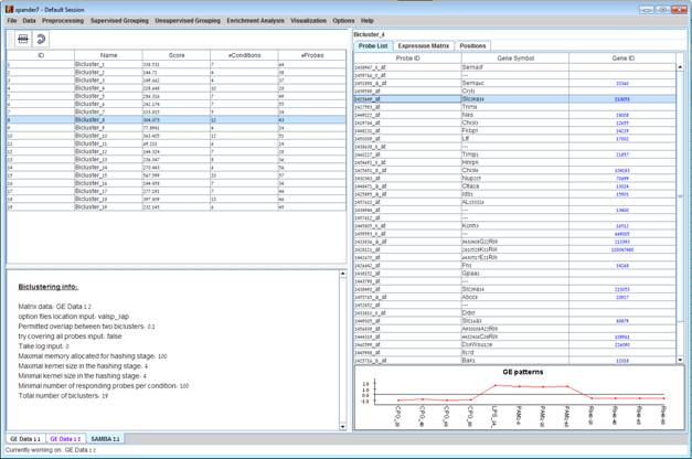
After biclustering is performed a biclustering solution visualization tab is added to the main window. It contains the following views:
a) Information regarding the biclustering algorithm, and number of resulting biclusters.
g)
Biclusters table – contains
the following information for each bicluster: serial number, name, score,
number of probes genes and number of conditions. The name of a bicluster can be
changed by editing the corresponding cell in the table. The score is given by
the SAMBA algorithm and is size-dependent, thus, it is not recommended to use
it to compare the quality of two biclusters of different sizes. The table can
be filtered to display a subset of the biclusters by clicking on the ‘Filter’ (![]() ) button in the
toolbar. Filtering can be performed according to: Score, number of probes and
number of conditions.
) button in the
toolbar. Filtering can be performed according to: Score, number of probes and
number of conditions.
Upon selecting a bicluster (from the biclusters table), the corresponding pane is displayed on the right. It contains a list of probes, probe patterns, expression matrix (heat map) and the chromosomal locations of the genes. Similarity matrices for probes within the cluster as well as for conditions are also displayed in this tab, if the relevant options in the display settings are selected (see the Settings section). If a network file has been loaded (via Data>>Load Network), the sub-graph, induced by the cluster is also displayed in the cluster pane.
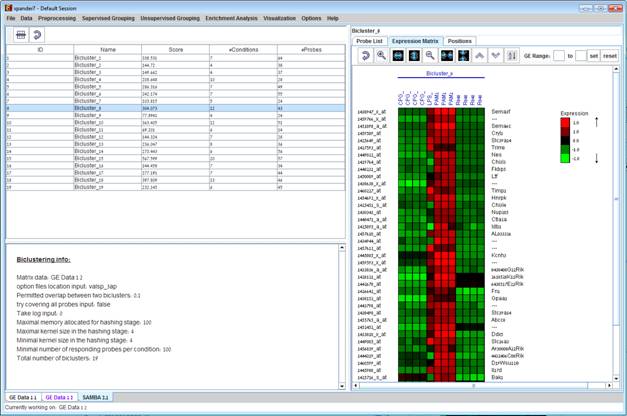

After performing enrichment analysis (for details see the Enrichment Analysis Tools section), if enrichment has been detected in the selected bicluster, the corresponding histogram and analysis information are added to the single bicluster view, and a column is added to the expression matrix display for each enrichment class, stating for each probe, whether it belongs to that class.
A biclustering solution can be saved using the File >> Export to text option (with the corresponding biclustering view as the selected tab) OR by using the File>>Save All option, which will export all solutions within a session to text and image files. A biclustering solution can be reloaded by selecting Unsupervised Grouping >> Bi-Clustering >> Load Solution. For a format of the solution file, please refer to the File Formats section: