MATISSE User Manual
Installation & Execution
Prior to installation please make sure that Java JRE version 5.0 or higher is installed at your computer. Java JRE is available here. Unzip the installation file matisse.zip into a directory of your choice. Use MATISSE.bat to activate the program. If your computer has more than 2GB RAM, use MATISSE_2GB.bat.
Getting started
Upon opening MATISSE, two options are available - to start a new session or to load an existing session.
If you select to start a new session, a start dialog is shown that allows you to load some data into the program. The initial specification includes the selection of the species and an option to load one interaction network and one expression dataset:
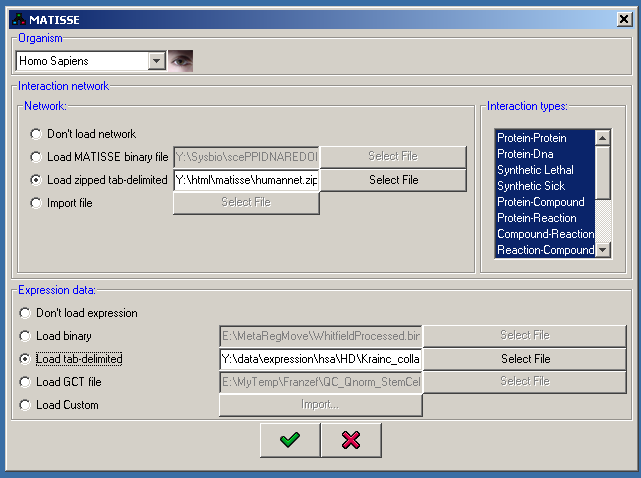
The first step is species selection, which is precondition for the other specifications. Currently the following species are supported:
 Homo sapiens
  Mus musculus
 Saccharomyces cerevisiae
 Drosophila melanogaster
 Caenorhabditis elegans
Note that the species selection affects the main identifier that should be loaded into the program in all the data files. For S. cerevisiae the expected identifiers are ORF names. For all other organisms MATISSE expects Entrez Gene identifiers.
It is also possible to select "Other species", in which case any identifiers can be used, but no additional information will be available for the genes.
For network loading the following options are available:
- MATISSE binary format
- MATISSE zipped tab-delimited format - examples for this format are available on MATISSE website.
- Import of interaction files - this brings up another dialog which allows you to import interactions in
the following formats:
- SIF format - Simple Interaction Format used by Cytoscape. This format is the one recommended for importing simple files. After loading the file, you will be prompted to specify the source of the interaction data. It is not obligatory to specify anything.
- BioGRID format - used by the BioGrid database (tab-delimited format).
- KEGG format - used the the KEGG database (tab-delimited format).
- Entrez Gene format - used by the Entrez Gene database.
You can also choose to skip loading the network right away and to load a network in a subsequent stage using the Load network command in the Network menu. In this case the program will be initialized with an empty network.
Expression data can be loaded either in the start dialog or afterwards using the Load expression data option in the Expression menu. For expression loading the following options are available:
- MATISSE binary format
- MATISSE tab-delimited format - a simple tab-delimited format in which the main identifier appears in the first column, a symbol (or anything else) in the second column and data entries in subsequent columns.
- Import of expression files - this brings up another dialog which allows you to import expression in
a custom tab-delimited format, while performing additional operations. This dialog contains the following tabs:
- File - allows the selection of the tab-delimited expression file and the specification of its exact format - it is possible to specify where (which row & column) the data entries are positioned in the file and which column contains the probe identifiers.
- ID matching - if the probe names in the expression file differ from the main identifier (ORF names for S. cerevisiae and Entrez Gene for others), it is possible to specify the conversion which has to be performed. The conversion file is a tab-delimited file with two columns - the first containing probe names and the second containing the main identifier.
- Probe - in case multiple probes with the same probe identifier are found in the file it is possible to specify how these are transfromed into a single pattern indexed by the main identifier.
- Filter - it is possible to specify which expression patterns will be used in the subsequent analysis. The filtering can be based either on the variation of the expression patterns or on the maximal value observed for the probe.
For expression data, note that if you intend to use the MATISSE algorithm, it is best to load data which is most suitable for computing Pearson correlations between gene patterns. If possible, it is best to provide log-ratios data. If the original data is Affymetrix or Illumina normalized ratio, they should be log-transformed (which can be done using the Expression->Transform dataset menu). Missing values can be estimated in MATISSE using the Expression menu.
Finding new modules
In order to find new modules using network and/or expression data use the  button in the main tool bar or the Find modules option in the File menu. Some algorithms are only available when network/expression data are properly loaded. Note that algorithms utilizing both network and expression data will only work if both data are loaded with matching identifiers (preferably with the default identifiers for the species in question, see above). Currently the following options are available for finding modules:
MATISSE
The MATISSE algorithm is relevant when both expression and network data are available. The following options can be adjusted:
- Expression dataset: The expression matrix used by the algorithm (relevant if more than one matrix is loaded when the algorithm is executed).
- Seed type: several seed type are available: All-neighbors/Best-neighbors/Heaviest subnetwork, as described in the MATISSE manuscript.
- Regulation priors: Also described in the manuscript.
- Beta: The parameter &betamates as described in the manuscript.
- Minimum/maximum seed size: The constraints on the seeds produced in the first phase of the algorithm.
- Minimum/maximum module size: The constraints on the modules produced in the second phase of the algorithm.
- Correlation type: The correlation statistic used to produced the pairwise similarities. It is recommended to use dot product (analogous to Pearson correlation).
Notes on using the MATISSE algorithm:
- Default parameters are expected to yield a reasonable performance, so they should be used first.
- Execution on more than 5000 front nodes can take a very long time or require too much memory.
- Prior to executing MATISSE, the expression data will be standardized (each gene pattern will be adjusted mean 0 and standard deviation of 1). Please make sure that the data does not contain missing values as this point.
CEZANNE
The DEGAS algorithm is described here. It is relevant when both expression and network data are available and when interaction confidence values are available. The options are largely similar to those in MATISSE. The only additional parameter is 'Confidence threshold' which specifies the q parameter of CEZANNE - the minimal confidence that at least one edge connects any two parts of a reported module.
DEGAS
The DEGAS algorithm is described here and it is relevant when both expression and network data are available and the expression dataset compares groups of hetherogenous samples (as in case-control studies).
Therefore it is possible to execute DEGAS only once at least one sample parameter with at least one value has been defined (using Expression->Define sample parameters menu).
The following options can be adjusted:
- Expression dataset: The expression matrix used by the algorithm (relevant if more than one matrix is loaded when the algorithm is executed).
- Sample parameter: The sample parameter used to distinguish between the 'case' and 'control' samples.
- Control parameter value: Samples with this value of the sample parameter will be treated as 'control' samples.
- Case parameter values: Samples with this value of the sample parameter will be treated as 'case' samples.
- Dysregulation direction: This parameter will determine which direction of dysregulation will be sought (up/down-regulation/both).
- Dysregulation significance threshold: This threshold will be used to identify which genes are differentially expressed in each 'case' sample compared to the controls.
- Optimization algorithm: The algorithm used to identify dysregulated pathways (DPs). See the DEGAS manuscript for details. CUSP is the recommended option.
- Starting points: Determines the number of starting points used by the optimization algorithm. Note that this parameter will heavily affect the running time of the algorithm.
- Minimum/Maximum tested k: The algorithm will try to identify DPs with different k parameter values (k determines the number of genes that are dysregulated in every sample). These parameters set the range of k that will be used.
- Tested k step: This parameter determines the interval at which different k values are tested.
- Random iterations for choosing k: The optimal k parameter is determined using randomization (see manuscript). This parameter specifies the number of random interations used. Note that it heavily affects the running time.
- l parameter: The l parameter specifies the number of allowed sample outliers (see manuscript for details).
- Maximum number of modules: After DEGAS identifies a significant DP, it removes it from the input data and attempts to identify additional DPs. This parameter specifies the total number of DPs that will be sought.
- Size p-value threshold for additional modules: This parameter specifies the threshold below which a DP will be considered significant, and additional DPs will be sought.
deMATISSE
The deMATISSE algorithm is described here. It is relevant when you are interested in identifying subnetworks of genes that are correlated with each other and also with some sample parameter. Therefore it is possible to execute DEGAS only once at least one sample parameter with at least one value has been defined (using Expression->Define sample parameters menu).
Most of the options are similar to those of MATISSE. The parameters specific to deMATISSE are:
- Sample parameter: The parameter that should be used for reference (the modules will be positive or negatively correlated with this parameter.
- Paramter type: Specifies if the parameter is numerical (e.g., age or tumour grade) or logical (e.g., healthy/sick, gender).
- Correlation with parameter: Specifies if the sought modules should be positively or negatively correlated with the parameter.
- Scale factor: Specifies the scale parameter which defines the relative importance of correlation with the parameter over co-expression (this is called Lambda in the text).
Custom MATISSE
This is a version of MATISSE in which the user can supplied a custom weight matrix (which should have both positive and negative weights).
Most of the options are similar to those of MATISSE. The only specific parameter is Weight matrix file that allows the user to specify the location of the weight matrix. The format of this file is very simple - it is a tab delimited table file, where the first row and column should correspond to gene identifiers (EntrezGene), or any other identifiers that match to the network nodes. A sample weight matrix file can be found here. All the genes which appear in the matrix will be considered as front nodes.
Co-clustering
The Co-clustering algorithm for simultaneous clustering of network and expression data is relevant when both of these data types are available. The following parameters can be adjusted:
- Expression dataset: the expression matrix used by the algorithm (relevant if more than one matrix is loaded).
- Number of clusters: the number of clusters produced (the algorithm is similar to K-means).
- Correlation coefficient: the correlation statistics used to compute the expression distances.
Expression k-means
The k-means clustering algorithm (applied to expression data). The following parameters can be adjusted:
- K: the number of clusters produced.
- Correlation type: the correlation statistics used to compute the expression distances.
- Matrix data: the expression matrix used by the algorithm (relevant if more than one matrix is currently loaded).
Expression t-test
This option applies the t-test to one of the loaded expression datasets. The following options are available:
- Expression dataset: the gene expression dataset to which the test will be applied.
- Sample parameter: the sample parameter according to which the two sample groups will be determined.
- Control parameter value: the sample parameter value with which the samples will be designated as 'control'.
- Case parameter value: the sample parameter value with which the samples will be designated as 'case'.
- P-value threshold: the threshold below which t-test results will be considered significant.
- Use ratio threshold: it is possible to use, in addition to the t-test, an additional threshold for the minimal ratio between the mean expression level in the case and control samples.
- Ratio threshold: the minimal ratio between case and control samples above/below which gene will be considered as differentially expressed.
- Multiple testing correction: the type of adjustment for multiple hypothesis testing. FDR refers to the Benjamini-Hochberg method.
CAST network clustering
This CAST algorithm for network clustering applied to the loaded network. The following options can be adjusted:
- t: the threshold parameter required by the algorithm (see manuscript for details)
- Minimum size: the minimum size of the modules which are reported.
- Minimum degree: the minimum degree of the nodes analyzed by the algorithm (required to reduce running time).
When all the options are adjusted use the  button to execute the module finder. After the module finding is over, a module set will be produced and the modules will be listed in a table in the upper left corner of the screen
Analyzing results
Every module set produced by a module finder or imported from an external file is represented within the program as a module set. The environment can maintain multiple module sets, but only one module set is the active module set at any given time. The active module set is selected in a drop-down list in the main toolbar. It is possible to add additional empty module sets using the Create new module set->Empty module set option in the Module set menu.
Once a module set is selected more options of the environment become available. This is an outline of the main window of the environment:
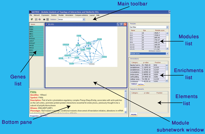
The main screen features available for analyzing modules are:
Module subnetworks area - In this area, module windows are presented. A window is opened for a module when in is selected in the modules list:
Modules list - in this table, all the modules in the active module set are listed. The table contains three columns: the name of the module, the number of genes it contains and an additional column (module attribute column), the contents of which are controlled by a drop-down list under the module table. This list contains all the module attributes which are available for the active module set. New attributes are added by some of the options which are described later.
By default all the modules in the active module set are listed in the modules list. It is possible to show only a subset of the modules by selecting a module filter from the roll-down menu above the list. The following filters are available:
- TANGO filter - it is possible to select a function, and only modules enriched with this function by TANGO are displayed.
- Annotation filter - it is possible to select an annotation from the active annotation database and only modules enriched with the annotation are displayed
- Gene filter - it is possible to select a gene, and only the modules which contain it are shown in the table.
- Interaction type filter - it is possible to select an interaction type (protein-protein, protein-DNA etc.), and only the modules which contain at least one edge of this types are shown in the table.
Selecting a module in the table makes it the active module and opens a corresponding module subnetwork frame in the Module subnetworks area.
Enrichments list - in this list its is possible to view different enrichments of the active module in two modes - the TANGO mode and the Annotation mode.
- TANGO mode - This mode displays the enrichments found by the TANGO algorithm which can be executed from the Annotation menu. The enrichments are presented in two columns: the name of the enrichment and the corresponding p-value. Note that p-values are corrected for multiple testing by resampling, and can not exceed 1/(number of resampling iterations).
- Annotation mode - This mode displays the annotations significantly enriched in the active module from the active annotation database. This database is selected in the Annotation menu, where it is possible to specify how the enrichment significance is evaluated. The enriched annotations are presented in three columns: the annotation name, the corresponding p-value and the fraction of all the genes tagged with the annotation within the module, out of the total number of genes tagged with the annotation.
Sequence elements list - This list is currently not supported in the public version of MATISSE.
Bottom pane
- In this pane two unrelated panels can be presented:
- Properties panel: in this panel, the properties of the current entity are presented. This view is changed following these actions:
- If the mouse is position over a node in the interaction network, the properties of the node are presented
- If a gene is selected in the gene list, its properties are presented
- If a module is selected in the modules list, its properties are presented.
- Sources panel: in this panel it is possible to browse the sources of the interactions in the active module subnetwork, and to choose which of them are visible (by using the appropriate check box). Selection of an interaction source colors all the interactions with this source in red. Note that interaction sources are grouped into a tree by their properties. The leafs of this tree correspond to individual sources. If the source is underlined - it can be double-clicked and the corresponding article in Pubmed is accessed.
Genes list
- This table contains a list of all the genes in the active module. The list can be sorted by the names of the genes in ascending/descending order by clicking the header of the table. Selecting a gene in the list paints it in white and scrolls the active module subnetwork window such that the corresponding gene becomes visible.
The module subnetwork window
After a module is selected in the modules list its subnetwork window opens in the module subnetworks area. This window presents all the genes (nodes) in the active module and the interactions between them.
The layout of the window is dynamic and it is possible to drag the nodes of the graph using the mouse left button. It is also possible to perform various layout operation, including automatic layout, from the Layout menu.
Note that directed edges generally correspond to protein-DNA interactions, and undirected ones to other types of interactions. Genetic interactions are denoted by green dashed lines.
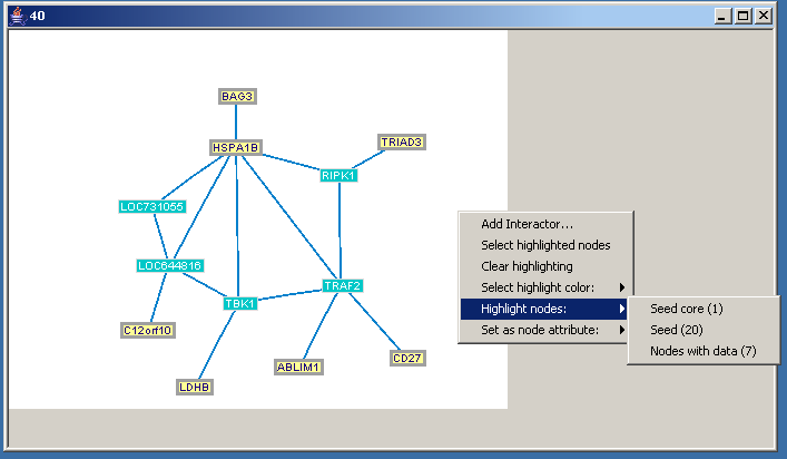
Additional operations are available in a pop-up menu that appears when the canvas is right-clicked:
- Add interactor - adds a new gene to the module, which is selected from a dialog which displays all the network nodes that are currently not part of the network.
- Select highlighted nodes - selects the nodes which are currently highlighted (how to highlight nodes is described later on).
- Clear interaction highlighting - resets the highlighting of the nodes.
- Select highlight color - selects which color will be used for the next highlighting.
- Highlight nodes - allows the highlighting of a subset of the module's genes, which have a certain node attribute (see below).
- Set as node attribute - allows to set a subset of the nodes as having a certain node attribute.
If a right-click is performed on one of the nodes it is possible to open a link to one of the databases that describe that gene. It is possible to get additional information by positioning the mouse over nodes/edges.
File menu: Saving and loading results
The best way to load/save results is through the "Load session"/"Save session" options in the File menu. Sessions are stored in a single .zip file that contains all the information about the network/expression data/modules/annotations.
In addition, it is possible to save all the active module sets into a simpler and smaller text file by by using the Save all module sets option in the File->Export module set(s) menu. Additional options available in the File menu:
- Import module sets - allows to load module sets from several formats:
- Import from MATISSE Loads module sets from a MATISSE file (generated using Save module sets.
- Import an Expander clustering solution - allows to load clustering solutions produced in the Expander software for microarray analysis.
- Load SAMBA biclusters - allows to load biclustering solutions produced by the SAMBA algorithm.
- Export module set(s) - its possible to export the gene content of the module sets in several formats
- Save all module sets - save all the available module sets in a simple light MATISSE format text file.
- Two columns format - exports the active module set in a two column tab-delimited text file (first column - identifier, second column - module name).
- Multiple single column files - exports the active module set into multiple single column text files (one per module).
- HTML website - builds a template of an HTML website containing the modules
- Import module - imports a simple gene list from a single column text file and adds it as a module to the active module set.
- Export active module - exports the gene list of the active module into a simple text file, or into Cytoscape SIF/GML files.
- Save interaction network - it is possible to save the active interaction network in a binary/tab-delimited/SIF format.
- Save expression matrix - it is possible to save the active expression matrix in a binary/tab-delimited format.
Network menu: Accessing network information
The Network menu has various options for handling network data loaded into the program:
Expression menu: Analyzing expression data
Once a module is selected and expression data is loaded it is possible to view the submatrix representing the expression values of the module's genes using the  button in the main toolbar. Details about this view are given here.
The Expression menu has the following options:
-
Load expression data - allows to load the expression matrix in ways similar to the ones available in the start dialog.
-
Switch active expression data - multiple expression matrices can be loaded, but only one can be analyzed at any given time. It is possible to choose the active matrix using this submenu.
- Rename dataset - changes the name of the active expression dataset (used for internal purposes).
- Remove dataset - unloads the active expression dataset.
- Define sample parameters - defines sample parameters - descripts of of the samples in the active expression dataset. The sample parameters can then be viewed in the expression matrix viewer or used as an input to the DEGAS algorithm.
- Show average patterns - displays the average gene expression pattern of a subset of the dataset - different options are available
- Calculate average correlation within each module- for every module, calculates the average correlation coefficient between the genes belonging to this module. Different correlation coefficients are available. The average value for every module is updated as a module attribute and can be viewed in the modules list.
- Show average correlation between modules- displays a similarity matrix which shows, for every pair of modules in the active module set, the average correlation between the genes that belong to different module sets.
- Transform expression dataset - several simple normalization methods are available through this submenu. More complicated transformations should be performed using the Expander software.
- Estimate missing values - estimates missing values in the dataset by: (a) replacing them with a constant value; (b) replacing them with the average expression pattern of the respective gene; (c) executing the k-nearest neighbours algorithm.
- Log(2) transform - applies log transformation to all the expression values.
- Standardize (mean 0, std 1) - transforms the expression pattern of each gene to mean 0 and standard deviation of 1.
- Show similarity between samples - displays a similarity matrix which shows, for every pair of conditions (columns in the expression matrix) the correlation coefficient between their expression profiles.
- Update symbols in the expression data - uses the gene database for the active species to update symbols in the expression dataset. The symbols can be viewed in the expression matrix viewer.
Module set menu
The following options are available in the Module set menu:
- Create new module set - adds a new module set. The new module set can either be empty, or formed for the modules in the active module set, each of which will be splitted into sub-modules using node attributes.
- Rename module set - renames the active module set.
- Remove module set - unloads the active module set.
- Show module set statistics - displays a summary of a few statistics about the active module set (number of modules, average module size etc.)
- Show module attributes - displays a table summarizing the module attributes for all the modules in the module set.
- Create new module - it is possible to add new modules to the active module set:
- Manually selecting genes - it is possible to select any genes that are found in the active species gene database. If necessary, the selected genes will be added to the active network.
- Using intersection of existing modules- generates a new module consisting of the intersection between the genes in several modules.
- Using union of existing modules- generates a new module consisting of the union between the genes in several modules.
- Using subtraction of existing modules- generates a new module consisting of the subtraction between the genes in one group of modules (which is selected first) and another group of modules (which is selected second).
- From an annotation set - generates a new module with all the genes in one of the annotation sets in a loaded annotation database.
- Show module overlap matrix - displays a similarity matrix displaying, for every module pair, the percent of the genes common to both modules.
- Show module overlap matrix - shows the overlaps between modules in the active module set.
- Remove selected module - removes the active module from the active module set.
Module menu
Options are available in the Module menu all refer to operations performed on the genes in the active module.
- Show module interactor summary - shows a summary of the genes in the current module (identifier, symbol, description and degree)
- Rename module - changes the name of the active module.
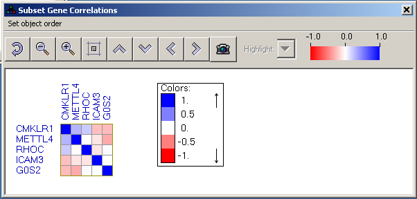
- Show expression similarity between genes - displays a similarity matrix displaying, for every pair of genes within the module, the correlation coefficient between their expression patterns.
- Show all annotations in module - shows all the annotations in the current annotation database that belong to an least one gene in the active module.
Annotation menu: annotating the modules
Two types of enrichment analyses of annotations are currently supported: (a) GO annotations using the TANGO algorithm which are corrected for multiple testing and annotation overlaps by random re-sampling; (b) annotations from different annotation databases which are not corrected for annotation overlap etc. (there are called annotations throughout the program and the manual) .
The following options are available in the Annotation menu:
- Switch annotation database - only one annotation database can be active at every time point. The selection in this submenu controls which annotations are presented in the enrichments list and in other views related to the enriched annotations
- Load annotation database - an annotation database can be imported into the program and loaded from:
- From a tab-delimited file - a simple two-column tab-delimited text file (first column - gene identifier, second column - annotation name).
- Load remote annotation DB - loads an annotation database from the MATISSE website (different annotations are available for different species).
- Show annotation database summary - shows a dialog listing all the annotations in the active database and the number of genes they represent. Clicking at annotation set will reveal the genes it contains
- Export annotation sets - saves the loaded annotation sets is the chosen format.
- Significance settings - specifies the settings used for evaluating sifnicicance of annotation enrichments.
- Load background set - loads a background set against which the enrichment is evaluated.
- Switch background set - chooses the background set that is used for enrichment computations
- Change p-value threshold - specifies the p-value threshold below which an enrichment is considered significant and is reported.
- Multiple testing correction - specifies the method of correction for multiple hypothesis testing.
- Recompute enrichments- recomputes the annotation enrichments using the active annotation database and the specifies enrichment detection settings.
- Show enrichment matrix- shows a shows a 0/1 similarity matrix between modules within the active module set and the annotations they are enriched with. If a cell in the matrix equals 1 (blue cell), it means that the module is enriched with the annotation.
- Show enrichment summary- shows a dialog with a table summarizing all the enrichments found in the active module set.
- Calculate average functional similarity within modules- uses the Gene Ontology functional similarity and computes the average functional similarity between the genes in each module. This value is set as a module attribute and can be viewed in the module attribute column in the modules list.
- Show average functional similarity between modules- for every pair of modules A and B computes the average functional similarity between a gene in A and a gene in B.
- Calculate lowest p-value in each module - for every module, compute the lowest enrichment p-value for an annotation set in the active annotation database. This p-value is set as a module attribute.
Layout menu
In the Layout menu it is possible to control the layout of the genes in the active module subnetwork window. The following options are available:
- Starts automatic layout - starts the execution of the automatic layout algorithm for the active window.
- Stop automatic layout - stops the execution of the automatic layout algorithm for the active window.
- Align top/bottom/left/right - aligns all the selected nodes in the active window.
- Distribute vertically/horizontally - distributes with equal spaces the selected nodes in the active window.
Similarity matrix display
This display shows correlations/co-occurances between two groups of objects, or between objects belonging to the same group. One group of objects is presented as the rows of the similarity matrix and the other as the columns. The matrix cells are color-coded based on the similarity values. Blue indicates positive values and red negative ones. The scale of the colors is -1..1 by default, but if the similarity values exceed this region, the thresholds are scaled such that full blue and red colors represent the 90% percentile of the value range.
Using the toolbar of the similarity matrix view it is possible to zoom in/out of the view and to shift the matrix in order to allow a better visibility of the row/column labels..
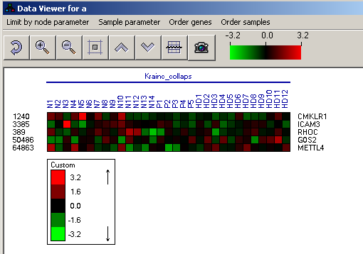
Expression matrix display
This view presents the expression values of a list of genes (rows) in a series of conditions (columns). The color scale can be set by clicking the color scale in the tool bar. It is also possible to adjust the view (zoom in/out etc.) using the toolbar.
For any questions, contact Igor Ulitsky
Back to the MATISSE homepage