ADEPTUS contains more than 14,000 ready to use gene expression profiles, each manually annotated to its most specific disease ontology terms.
For getting the expression profiles, sample labels, gene scores and more see the Download page.
In the table at the bottom of this page you can get the implementation of useful R functions. To analyze the data follow this tutorial script.
The code first loads all required libraries, data and functions required.
Afterwards, there are two types of analyses that you can perform: generate classification results (part 1), and integrative analysis of the discovered gene sets with mutation, drug-target,
and pathway data (part 2). Below we give more details on each part.
Using the first part of the R tutorial script you can perform your own leave-dataset-out cross validation (LDO-CV). Using this analysis you can detect well classified diseases. In addition, you can train a classifier and test it on another dataset. For example, you can use the classifier that was learned on all microarray samples and test it on the RNASeq samples.
In the second part of the tutorial you can analyze discovered disease gene sets with external data. For each disease, the output of the code is a file with
a gene set and its attributes that can be analyzed in Cytoscape . The required Cytoscape Apps are
GeneMANIA, and EnhancedGraphics .
To generate a disease-specific summary map:
1. Load the gene set into a GeneMANIA search, use only protein and genetic interactions.
2. Load the file (the output of the R script) as an attribute file for the nodes.
3. Make sure you use gene names in the relations when uploading the file (GeneMANIA's default labels are other ids)
4. Create a custom graphics property for the nodes (using "Chart 2" as a passthrough mapper, see the script).
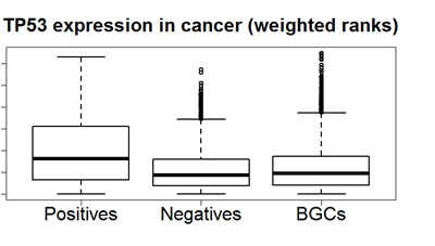
As an example of a disease-specific differential gene, consider the expression pattern of P53 in cancer.
The y-axis represents the rank-based expression of the gene across samples. Positives are cancer patients, negatives are healthy controls, BGCs have some non-cancer disease.
Thus, P53 is significantly (p = 1.2E-12) up-regulated both when compared to negatives and BGCs.
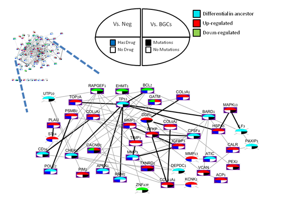
The integrative analysis in part 2 of the tutorial code uses mutation profiles from COSMIC, drug information from DrugBank, and gene-pathway mapping.
The output is a table in which each row represents the information of a gene. By uploading the data into Cytoscape as explained above, you can create summary
maps similar to the example below (lung cancer). In large maps manual rearrangement might be required for improving visibility.
| Name (link) | Description | Dependencies |
|---|---|---|
| Tutorial | A tutorial on how to use our code and data for generating results. For example, running LDO, or creating data for analysis in Cytoscape (e.g., creating Figure 6) | Explained within |
| GEO data retrieval functions | Wrappers of functions of GEOquery used to get the data of a set of dataset identifiers | GEOquery |
| Functions for DO structure analysis | Simple methods for analysis of the DO structure and methods for getting the underline Bayesian Network from a set of DO IDs (used for Bayesian correction) | BNlearn, DO.db |
| Helper methods for GE preprocessing | Methods that were used when mapping the original GEO data to Entrez (using the platform data object above) | BiomaRt, hash |
| Helper methods for GE analysis | Auxiliary methods for GE analysis, e.g., rank-based normalization and quantile normalization | QEOquery, hash |
| Classification methods | Methods for standard classification | CMA, e1071, RandomForest, limma, ROCR |
| Multilabel classification methods | Methods for multilabel classification (e.g., Binary relevance, LP, Bayesian Correction) | BNlearn, Classification methods |