Gene expression measurements using cDNA microarrays do not provide absolute mRNA levels in a single condition of interest, but only relative mRNA levels in pairs of conditions. Hence, an experiment gives for each gene the ratios of its mRNA levels in a test and reference conditions. In order to use such data in our analysis, we first have to transform experiments into absolute mRNA levels in single conditions and then use them to evaluate model discrepancy. This can be easily done if all experiments are using a common reference condition. In this simple case, we may directly use the relative measurements as the observed states in the test condition, due to the fact that all relative measurements are comparable.
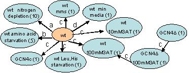
In practice, not all experiments use the same reference condition. To handle this case we define the experiments graph , a directed multigraph in which vertices represent conditions and arcs represent experiments. For each experiment, we add an arc from the reference to the test condition vertex. Note that condition vertices can be reused. Let l(v,i,j) be the logarithm of the ratio of gene v's levels in condition i and condition j. For gene v, the weight of arc (i,j) is precisely l(v,i,j), as obtained from the microarray in the experiment with test condition j and reference condition i. We wish to compute a normalized log hybridization level (we will refer to it as level ) for each mRNA variable in each condition. Assume first that the graph is connected. The idea is to fix one vertex in the graph as a common reference and compute the levels of all other conditions relative to it. We then discretize the levels to generate the observed states of each condition.
Our normalization procedure works as follows: First, using prior biological knowledge we fix the levels of the mRNA variables in one condition (the source condition). Second, we use a breadth-first search algorithm on the underlying undirected experiment graph in order to handle condition vertices by an ascending distance from the source condition. When reaching a condition i, there must be at least one neighbor whose levels are already determined. We compute the level of each mRNA variable v in the condition i as follows: The contribution of an incoming neighbor j is defined as l(v,j) + l(v,j,i) where l(v,j) is the level of variable v in condition j. For an outgoing neighbor j, the contribution is defined as l(v,j) - l(v,j,i). We compute the level of v at condition i by averaging the contributions of all determined neighbors. In case more than one connected component exists, we must fix a common reference in each component and ensure their levels are comparable. Note that if we have absolute measurements on more than one condition in a connected component of the experiment graph, the algorithm can be adapted to take this information into account.
In order to calculate the observed states for our datasets, we created the experiment graph (below). We used growth of a wild-type strain in standard conditions and YPD medium as our source condition, and fixed its levels to 1 for all genes. We assigned the computed levels in the range (-inf,0),[0,2) and [2,in) to the observed states 0,1 and 2, respectively.
Protein data
The observed states of proteins in minimal media were obtained by discretizing the concentration levels reported by Washburn et al. (2003). We assigned the values in the range [0,0.5],(0.5,1.5], and (1.5,inf) to the observed states 0,1 and 2 respectively.
Phenotype data
The observed states of the growth phenotypes were obtained by discretizing the sensitivity scores reported in Giaever et al (2002). Giaever et al. (2002) computed for each strain and environmental condition a sensitivity score, and assigned the sensitivity scores in each generation time a cutoff of significance. Following these cutoffs, we discretized the sensitivity scores in the range [0,10],(10,20], and (20,inf) to observed states 0,1, and 2, respectively for 5 generation phenotypes, and [0,20],(20,100],(100,inf) for 15 generation phenotypes. The growth phenotype was associated with the level of the internal lysine variable in the model.
* A. P. Gasch et al. Genomic expression programs in the response of yeast to environmental changes. Mol Biol Cell, 11:4241 57, 2000.
* K. Natarajan et al. Transcriptional profiling shows that GCN4p is a master regulator of gene expression during amino acid starvation in yeast. Mol. Cell. Biol., 21:4347 4368, 2001.
* M.P. Washburn. Protein pathway and complex clustering of correlated mRNA and protein expression analyses in S. cerevisiae. PNAS, 100:3107 3112, 2003.
* G. Giaever et al. Functional profiling of the S. cerevisiae genome. Nature, 418:387 391, 2002.