Installation and Execution
After downloading MetaReg.zip and extracting it, use metareg.bat for execution in Windows and metareg.csh for execution in Linux. When running on Linux/Unix OS, make sure that you have rwx permissions for the MetaReg directory and for the directory in which your data is located.Model definition
Defining a new model
Pressing in the main toolbar or using New... in the File
menu initiates the design of a new MetaReg model by opening the Model Definition dialog.
in the main toolbar or using New... in the File
menu initiates the design of a new MetaReg model by opening the Model Definition dialog. For each model, the following details can be specified (Figure 1):
- The name of the model.
- The name of the model author.
- The species the model refers to.
Saving and loading models
Models can be saved ( ) and loaded (
 ) from
flat text files. Both commands are accessible from the File menu and from the main toolbar.
All the loaded data and attributes are saved along with the model definitions.
All the data relevant to the model is stored in a single tab-delimited text file, the format of which
is described here .
) from
flat text files. Both commands are accessible from the File menu and from the main toolbar.
All the loaded data and attributes are saved along with the model definitions.
All the data relevant to the model is stored in a single tab-delimited text file, the format of which
is described here .
Saving and loading sessions
The set of all the currently available models along with the corresponding prediction results can be saved as a single session. Sessions can be saved ( ) and loaded (
 ) from
zip archive files. Both commands are accessible from the File menu.
) from
zip archive files. Both commands are accessible from the File menu.
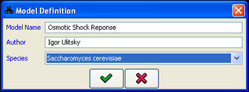
Figure 1:Model definition dialog
Defining Model Variables
A MetaReg model is defined by a set of its variables and their discrete logics. The first step in defining a MetaReg model is thus the definition of the variables participating in it.The addition of variables to the model can be done by right-clicking the model canvas or through Add variable in the Model menu. After the variable has been added to the model, its properties can be edited by double-clicking it on the model canvas, or by right-clicking the variable and picking the Edit Variable option. The manipulation of all the variable properties and most importantly its logic are done through the Edit Variable dialog (Figure 2). This dialog is used both for defining new variables and adjusting existing variables. The variable properties are divided into 4 separate tabs: General, Logic, References, Expression Table, each of which will be elaborated below:
1. General variable properties
The following properties can be adjusted in the Properties tab. Some of the values can be automatically filled using the gene library.
- Name: The name of the variable as it will appear in MetaReg. It is advised that this name consent with the name of the variable in the imported data, unless another Id is provided. In case several variables represent the same gene (e.g. an mRNA variable and an active protein variable), it is a good practice to name the variables accordingly (e.g. mRAP1 and apRAP1).
- Id: The external id that, if specified, will be used for matching the variable against the imported experimental data.
- Description: A general description of the variable.
- Type: The type of the variable. Currently the following types are supported:
- mRNA
- Active protein
- Inactive protein
- Internal metabolite
- External metabolite
- Phenotype
- Other
- Cardinality: The cardinality of the variable is the number of different logic states it can attain
in the model. The default cardinality is set to 3, usually used to represent the states of:
- 0 = down regulation
- 1 = normal state
- 2 = up regulation
- Aliases: Additional names for the variable can be specified here.
- Uncertainty: The user can specify the uncertainty in the regulation logic of the variable. This uncertainty value is used in the probabilistic prediction execution.
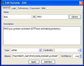
Figure 2:Edit Variable dialog
Adding variables from the gene library
For defining variables describing known biological entities the user can utilize common domains containing extensive gene-based information. Currently, for S. cerevisiae all the genes from Saccharomyces Genome Database (SGD) can be selected. For all other organisms, the listings are available from the Entrez Gene database.When defining entities through this dialog, the name, id, description and aliases of the variable are automatically added to the variable properties. The Gene Library dialog (Figure 3) can be accessed using the Library button. A gene can be sought using either its official name or on any one of its aliases specified in the listings. All the relevant information for each entry appears in the Properties panel.
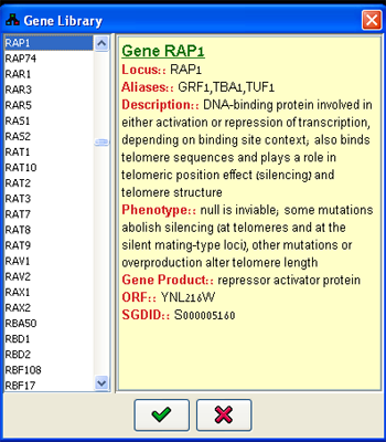
Figure 3:Gene Library dialog
2. Variable regulation function logic
Defining the regulation logic for every variable is the most difficult step in model formulation. In order to facilitate this modeling stage, several gadgets exists in the application for logic definition:Scripting logic
The advanced users can enter the logic function using a script. The script represents the logical function using simple notation and bracketing.The script can contain the following:
- Constant values (e.g. 0/1/2/…)
- Names of model variables.
- Simple logic functions: Min() ,Max() and Sum().
- For complex logic functions, The script can contain the Table[ ]() function, where the target variable values for each input combination are entered within the [,] brackets and separated by spaces.
The following tools can be used in the scripting process:
- The basic functions Min, Max and Sum can be added to the script using the respective buttons
- The name of any variable in the model can be selected from a combo box and added using the Insert button.
- Table logic can be edited by first adding the command Table[](Regulator1,Regulator2) to the script, with the correct regulators of the variable, and when using Edit Table... button (which will becomes enabled when a table entry in the script is selected by double-clicking the word Table in the script). Editing the Target Variable column in the Edit Table dialog will affect the script accordingly.
- Special types of common table logic can be added by using a Conditional Logic Editor, which can be accessed through the If... button.
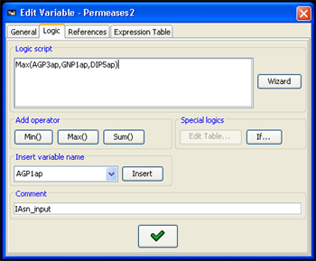
Figure 4:Logic editor
Logic Editor Wizard
A more intuitive way to edit the logic is through the logic editor wizard, which exploits the tree structure of the logic function. The wizard works in conjunction with the script editor - the current script will be displayed when the editor is accessed using the Wizard button in the logic editing panel, and when the editing is concluded, the script will be updated based on the logic generated by the wizard.
Within the wizard, all the variables in the model are displayed in the Variables list. The constructed
logics are displayed as hierarchies in the Logics panel. It is possible to maintain several logics
during the editing, but only a single entry in the tree will have to be selected when the editing is done.
All the other logics will be discarded after  is pressed.
New logics can be created by one of the following:
- A simple equals to another variable logic can be added by selecting a variable from the variables list and using the Add button in the Regulators panel.
- A constant logic can be added by selecting the desired constant in the Constants panel and using the Insert button.
- Several logic can be combined by selecting them in the Logics panel (keep Ctrl pressed while selecting for multiple selection), and then using the Min(),Max(),Sum() or Table() buttons in the Add Logic panel. This will add the a new logic with the requested operator and the selected logics as its inputs. Using Table() will automatically open the table logic editor for editing of the table values.
Using the tools described above, a simple Min(varA,varB) can be constructed using the following workflow:
- Select varA in the Variables list and add it to the logics using the Add button.
- Select varB in the Variables list and add it to the logics using the Add button.
- Select both varA and varB in the Logics list, while keeping the Ctrl key pressed.
- Use the Min() button.
- Select the Min(varA,varB) logic which now appears in the Logics list.
- Press
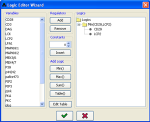
Figure 5:Logic editor wizard
Conditional Logic Editor
Conditional logic is a logic of the type If A then B, otherwise C. This kind of logic can be created by pressing the If... button in the logic editor. This opens the conditional logic editor dialog. The condition (e.g. GCN4=2 or RAP1>0) can contain any logic, a conditional operator (<, >, or =) and a constant. The If true and If false fields can contain any logic script. When
is pressed, a table logic corresponding to the requested values is automatically generated.The if A then B, otherwise C structure of the logic will be recorded in the Comment field in the logic editor.
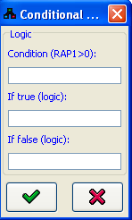
Figure 6:Conditional logic editor
3. Variable references:
Each variable can be attributed with references to journal publications, in order to facilitate further model curation and to organize the published results supporting decisions made about properties and logics. The references can be obtained using on-line search of PubMed dialog accessible through the References tab.
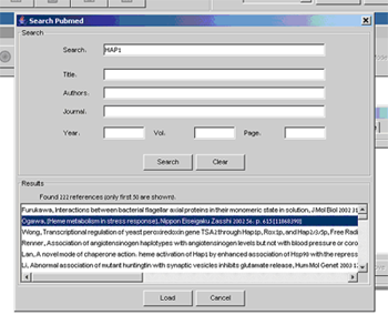
Figure 7:Add Reference dialog
4. Experimental data table:
After experimental data is imported to the model, this tab shows a table of all the raw values for this variable. It is not possible to perform any changes to the data using this table.
Handling model frame visualization
Several models can be handled concurrently in the application. The currently active model is defined by the selected model frame. The title of the frame indicates the name of the model, along with the file associated with it (if one exists).The model graph display is fully dynamic and the nodes and edge centers are draggable. In order to drag an edge, use a small point at its center. In addition, the following features are available in the display:
Node alignment
It is possible to align the positions of nodes on the graph by first selecting them and then using the alignment options in the Layout menu.Node highlighting
It is possible to highlight specific nodes be selecting an appropriate option in the Highlight list in the model frame toolbar. It is possible to highlight all the nodes on cycles, the current feedback set, different variable types, and the perturbed nodes in the data/simulation.Variable pop-up menu
Right-clicking any node on the graph brings up the variable pop-up menu. The following options are available:- Edit Variable... - opens the variable editor dialog (same as in adding the variable).
- Lock Location - fixes the variable position when using automatic layout.
- Remove Node - removes the node from the model. Notice that removing a variable with regulates other variables can affect their logic.
- Simulated Perturbation - in the simulation mode, this option can be used for specifying perturbations.
- References - when references are added to the variable, it is possible to access them directly through this menu.
- Web Info - Opens a relevant web page describing the gene represented by the variable (if one can be matched by its name/ids).
Model canvas pop-up menu
Right-clicking on an empty space inside the model frame brings up the model canvas pop-up menu. In this menu it is possible to use the Add Variable... option to add variables to the model.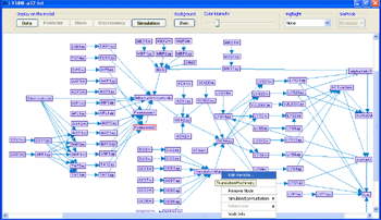
Figure 8:Model layout
Performing simulations
After a model is partially specified, it is possible to simulate the values of all the variables under a set of simulated perturbation. The simulation utilizes uses discrete inference, as described in the MetaReg JCB 2004 paper.The simulation mode can be toggled by pressing the Simulation button in the model frame. This will automatically display the current simulated values, represented by numbers adjacent to the variable nodes. The values are color-coded: 0 with a green background and any value = 1 with a red background. If no feasible mode is found, no number will be displayed. If more than one mode is possible, different modes can be navigated using the SimMode menu.
It is possible to specify a simulated perturbation by using the variable pop-up menu. The simulation values are automatically re-computed after any change to the model or the perturbations. Notice that a large feedback set of the graph might results in poor performance in the simulation mode.
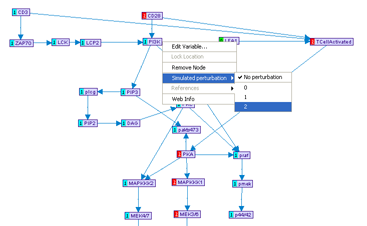
Figure 9:Simulation mode
Importing external measurement data
The data import can be accessed through Load experimental data ( )
button in the main tool bar, which opens the Import data dialog.
)
button in the main tool bar, which opens the Import data dialog. Currently, only import from tab-delimited files is supported.
1. Adjusting the correct file format
Within the dialog, first select a file in the File panel. File selection automatically loads the first 20 lines in the file for preview purposes. If the file is loaded correctly, the heading row and column and the data contents will be painted in different colors. Otherwise, all the content of the preview panel will show with red background.The parsing of the file structure can be configured through the Attributes panel. The Entry Id column attribute refers to the column whose content will be matched against the names/ids of the variables in the model. The Attributes column refers to the column which can contain two meaningful values: "E" indicates that this column contains information about a perturbation performed in the specified condition; "M", on the other hand, indicates that this column contains measurement data. Notice that values in the "E" rows are expected to contain "logical" values (e.g. 0/1/2), while the values in the "M" rows are usually continuous measurements. For example, if the data contain microarray gene expression measurements of four genes: geneA,geneB,geneC and geneD, one with geneA knocked-out, one with geneB overexpression and one with both perturbations, the table should look like this:
| Gene | Attribute | Condition1 | Condition2 | Condition3 | |
| geneA | E | 0 | 2 | ||
| geneB | E | 2 | 2 | ||
| geneA | M | -3.2 | 0.6 | -0.4 | |
| geneB | M | 1.2 | 4.1 | 1.1 | |
| geneC | M | 3.2 | -1.2 | -1.3 | |
| geneD | M | -2.4 | 2.0 | 0.3 |
If the None is selected for Attribute column, all the rows will be treated as measurement rows. In any case, the condition attributes can be assigned later on. Note that if multiple rows are found for the same identifier, their values will be averaged.
After all the attributes are correctly set, and the preview is colored correctly, pressing the Load button causes the program to import all the file and enable the Relativities, Variable Matching, Preprocessing and Perturbations tabs. These can be used to customize the translation of the data in the imported file into Conditions within MetaReg.
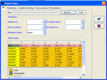
Figure 10:Adjusting the imported file format
2. Adjusting condition relativities
By default, if no adjustment is performed in the Relativities panel, all the conditions in the imported file are treated as quantities measured relative to some WT_CONDITION, in which all the variables equal 0.If this is not the desired case, for example, if every value should be treated relative to a value in the previous condition, the relativities can be selected in the Experiments table, adjusting the Ref and Test columns. The eventual values used in every condition will be generating by subtracting the values value in the Ref column from the value in the Test column. If necessary, additional condition names can be entered in both the Test and the Ref columns. Conditions can be excluded from the import process by unselecting their respective check-boxes in the Use column.
The relativities adjustment process has to start from some initial condition, whose values will be automatically set to zero for all variables. By default, this is the automatically added WT_CONDITION. Any other condition can be selected for this purpose (e.g., point 0 in a time series), using the Base condition panel, which contains the name of all the experiments (columns) in the imported file.
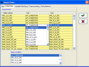
Figure 11:Adjusting condition relativities
3. Matching row names in the file with variables
In order to correctly assign the measured data to the model variables, a matching has to be made from the row names in the file (entry id column) to the names of the variables in the model. This matching can be adjusted using the Variable matching panel. The program attempts to automatically perform this matching using the Id property of the variable. If no such property exists, the matching is attempted using the name of the variable. If this fails, the gene library for the species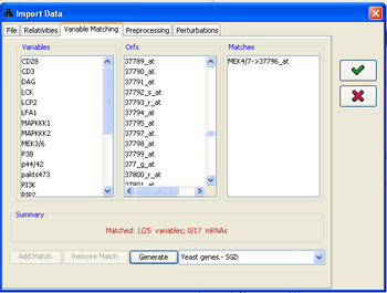
Figure 12:Matching file rows to variables
4. Specifying condition attributes
If the supplied data file doesn't contain all the information about the perturbations performed in every condition, or contains only part of it, this information has to be specified within the program. The condition attributes are used in the probabilistic prediction engine and are displayed along with the rest of the data.
The attributes can be specified as part of the data import process in the Attributes tab of the import
dialog. The Conditions panel contains a list of all the conditions currently loaded. Any subset of the
conditions can be selected (for multiple selection keep the Ctrl key pressed). Following every selection,
the Attributes panel is set to display/edit the attributes common to all the selected condition subset.
When multiple conditions are selected, only attributes common to all the conditions are displayed. Attributes can be added using
the  button and removed using the
  button. In every row in the table both the perturbed variable and its state can be altered. The changes are
instantaneously performed. The same panel can be used later for altering the conditions, as described in the
Data visualization section.
button. In every row in the table both the perturbed variable and its state can be altered. The changes are
instantaneously performed. The same panel can be used later for altering the conditions, as described in the
Data visualization section.
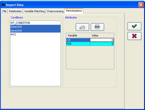
Figure 13:Specifying condition attributes
5. Finishing the import process
After all the import details are specified, pressing closes the import dialog
and generates new conditions. Notice that importing data does not erase previously loaded conditions, but rather
appends the new ones to the existing list.
Organizing the experimental conditions
After conditions are imported it is possible to further adjust their properties by accessing the condition organizer using the button in the toolbar. The organizer allows the following operations:
- Reordering of the conditions: using the
 and
and  buttons.
- Deletion of conditions: using the
 button.
- Setting the attributes (perturbations) to a set of conditions, by selecting them while Ctrl is pressed and then adding/removing attributes, as described in the import process.
- Adjustment of the value thresholds used for the visualization of the condition data in the data matrix viewer.
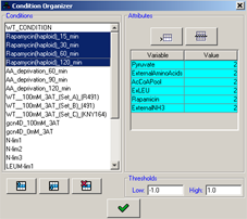
Figure 14:Organizing the conditions.
Data visualization
Viewing data on the model graph
After conditions are imported, the conditions toolbar, located right below the main toolbar becomes activated. It is possible to project one condition at a time on top of the model graph. In order to do so, select a condition using the Condition list in the conditions toolbar, and then toggle the Data button in the model frame toolbar. Doing so will present a new bar over every variable with an observation in that condition. The conditions can than be navigated through the conditions list. The values are color-coded: red represents positive values and green negative ones. The color intensity can be adjusted using the Color intensity slider bar. The actual value of every observed variable can be viewed by positioning the mouse over the color label. It is also possible to switch the background of the model frame to black through the Background panel.
It is possible to remove conditions from the model by using the  button, and
to remove all the conditions at once using the
button, and
to remove all the conditions at once using the  button. Pressing
 open a dialog for editing the attributes of the current condition. This dialog
is identical to the panel described in setting conditions attributes section.
Pressing
open a dialog for editing the attributes of the current condition. This dialog
is identical to the panel described in setting conditions attributes section.
Pressing  toggles the visibility of the matrix data display.
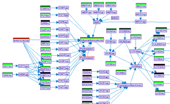
Figure 15:Visualizing data on the model canvas
Viewing data using the matrix data viewer
Activated from the conditions toolbar, the matrix data viewer provides a simultaneous display of all the available conditions. The matrix rows are all the variables with at least one observation/perturbation in the data, and the columns are all the available conditions. A missing cell in the matrix is represented by a black color. A legend for the other cell colors appears below the matrix.It is possible to re-order the variables in the matrix based on their values in the specific condition by clicking on the name of that condition in the matrix. Perturbations are denoted by a black stripe in the upper portion of the respective matrix cell. On top of the matrix a bar contains information about the name of the file that the data was derived from. Positioning the mouse above a cell presents its values.
The toolbar of the Data Table Viewer dialog contains several view manipulation options.
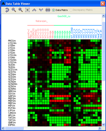
Figure 16:Visualizing data using the matrix viewer
Prediction execution
When the model is defined and some conditions with attributes are described, it is possible to use the probabilistic prediction engine to infer the values of all the variables in the model in all the available conditions. Note that the prediction engine computes predictions based on the model and the data perturbations, but ignoring the measurments.
The prediction engine execution dialog can be accessed through  in the main toolbar.
The different prediction algorithms are described in the
FGN article. The recommended algorithm for this task
is LBP. It is important to make sure that the feedback set for the model is correct and as small as possible. How
update the feedback set is explained here.
in the main toolbar.
The different prediction algorithms are described in the
FGN article. The recommended algorithm for this task
is LBP. It is important to make sure that the feedback set for the model is correct and as small as possible. How
update the feedback set is explained here.
All algorithms require the specification of a single connected component in the network on which the predictions will be performed. This selection is done in the Subset focus panel.
to execute the prediction algorithm.
If the execution terminates successfully, you'll be asked to specify a name for the results set. This name
will be used to designate the current results set. It is possible to maintain several result sets, e.g. using
different parameters, or different logic functions. It is not advised to maintain different results set after
more drastic model changes such as variable removal, as it might provide with unexpected results.
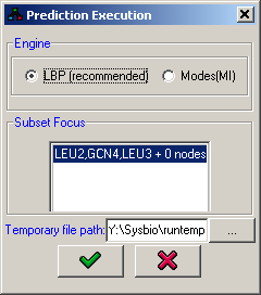
Figure 17:Prediction execution
Analysis of prediction results
Prediction results can be analyzed after a successful prediction execution, or after prediction results are loaded using the button. In any case, the desired results set can
be selected in the Prediction results: list in the results toolbar. The selected results set can be removed
using the Remove button and all the sets can be removed using the Clear button.
button. In any case, the desired results set can
be selected in the Prediction results: list in the results toolbar. The selected results set can be removed
using the Remove button and all the sets can be removed using the Clear button.
Displaying predicted values on the model graph
Predicted values can be displayed on the model graph by toggling the Posterior button in the model frame. Alternatively, discrepancies between the posterior and the measured values (where available) can be displayed in a similar way using the Discrepancy button. The Mode button is useful only in case the MI algorithm was used for the prediction task. In which case it can be used to toggle the view of mode information.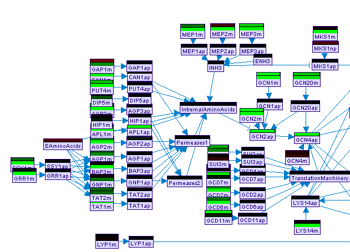
Figure 18:Display of observed values and prediction posterior on the model frame
Discrepancy matrix
In the matrix data display it is possible to the select the Discrepancy matrix display to view the discrepancies between the measurements and the predicted values in all the conditions. The discrepancy matrix display is similar to the data matrix, but every cell contains a color-coded representation of three values - the cell background represents the difference between the observed and the predicted values, the left small square represents the measured value and the right small square the predicted one. The tooltip text showed when the mouse is delayed over a matrix cell contains the full information about the exact values corresponding to the cell.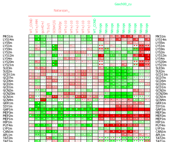
Figure 19:Discrepancy matrix
Refinement execution
It is possible to use the probabilistic engine to refine the logic of a specific variable for a pre-defined set of parents. The refinement can be executed using the button in the main toolbar. In the dialog that will
appear you'll need to specify the variable whose logic will be refined and select its parents from the variable list using the
button in the main toolbar. In the dialog that will
appear you'll need to specify the variable whose logic will be refined and select its parents from the variable list using the
 and the
  buttons. It addition, it is necessary to specify
the significance threshold, the likelihood ratio above which specific logic entry will be considered significant.
Make sure to specify a valid directory for the placement of the temporary files produced by the refinement engine.
When all the configuration is set use the button to execute the refinement engine.
buttons. It addition, it is necessary to specify
the significance threshold, the likelihood ratio above which specific logic entry will be considered significant.
Make sure to specify a valid directory for the placement of the temporary files produced by the refinement engine.
When all the configuration is set use the button to execute the refinement engine.
When the refinement process terminates, the newly learned logic is presented in a table logic editor, where it can be further adjusted, by setting the values in the "Target variable" column. The values in this column are color-coded based on the values of the learned logic. In addition, the "Meaningful" column specifies whether every entry in the logic learned is significant given the threshold specified in the configuration. The means of the actual data values that were learned for each discrete value are shown on the bottom.
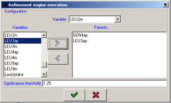
Figure 20:Configuration of the refinement execution
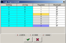
Figure 21:Table logic learned by the refinement engine.
Miscellaneous
Model file format
A full description of the model file format is available here.Specifying the feedback set
Both simulations and prediction require the correct definition of the feedback set in the model graph. MetaReg attempts to maintain an optimal size feedback set by an exhaustive algorithm which assumes that the size of the feedback set is small. If the user wishes to specify a different feedback, the Edit feedback set
option can be accessed from the Model menu.
Edit feedback set
option can be accessed from the Model menu.
In the dialog, the current feedback set is displayed as a list of variables. This list can be modified
using the Remove and Clear buttons. New variables can be added to the feedback set using
the Variables panel. After pressing , the system will validate that
the graph without the current feedback set does not contains cycles. It is not possible to proceed further while
the feedback set is not valid. Notice that a large feedback set results in a poor performance of all algorithms.
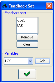
Figure 22:Feedback set editor
Additional display options
Bird eye's view
A high-level image of the model can be toggled through in
the main toolbar.
in
the main toolbar.
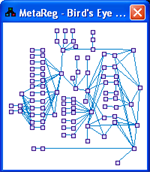
Figure 23:Bird eye's view
Properties display
Using in the main toolbar, the properties display view can
be toggled. This dialog provides additional information about objects pointed by the mouse.
in the main toolbar, the properties display view can
be toggled. This dialog provides additional information about objects pointed by the mouse.
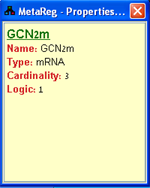
Figure 24:Properties display
Variable list
Using in the main toolbar, the variable list dialog can
be toggled. The variable list contains a dynamic listing of all the variables in the model. Selecting
a variable from the list highlights it on the model graph.
in the main toolbar, the variable list dialog can
be toggled. The variable list contains a dynamic listing of all the variables in the model. Selecting
a variable from the list highlights it on the model graph.
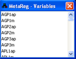
Figure 25:Variable list
Copyright information
Copyrights © Tel-Aviv University, Israel (2006).A portion of the user interface code is due to Sun Microsystems.Inc. Copyright 1994-2004 Sun
Microsystems, Inc. All Rights Reserved. The following license rules apply to
that portion:
"Neither the name of Sun
Microsystems, Inc. or the names of contributors may be used to endorse or
promote products derived from this software without specific prior written
permission.
This software is provided "AS IS," without a warranty of any kind.
ALL EXPRESS OR IMPLIED CONDITIONS, REPRESENTATIONS AND WARRANTIES, INCLUDING
ANY IMPLIED WARRANTY OF MERCHANTABILITY, FITNESS FOR A PARTICULAR PURPOSE OR
NON-INFRINGEMENT, ARE HEREBY EXCLUDED. SUN MICROSYSTEMS, INC. ("SUN")
AND ITS LICENSORS SHALL NOT BE LIABLE FOR ANY DAMAGES SUFFERED BY LICENSEE AS A
RESULT OF USING, MODIFYING OR DISTRIBUTING THIS SOFTWARE OR ITS DERIVATIVES. IN
NO EVENT WILL SUN OR ITS LICENSORS BE LIABLE FOR ANY LOST REVENUE, PROFIT OR
DATA, OR FOR DIRECT, INDIRECT, SPECIAL, CONSEQUENTIAL, INCIDENTAL OR PUNITIVE
DAMAGES, HOWEVER CAUSED AND REGARDLESS OF THE THEORY OF LIABILITY, ARISING OUT
OF THE USE OF OR INABILITY TO USE THIS SOFTWARE, EVEN IF SUN HAS BEEN ADVISED
OF THE POSSIBILITY OF SUCH DAMAGES.
You acknowledge that this software is not designed, licensed or intended
for use in the design, construction, operation or maintenance of any
nuclear facility."
For any questions, bugs and suggestions, please contact: Igor Ulitsky