Expander Online Documentation

 

Table of Contents

 

Introduction. 2

Starting EXPANDER. 2

Input Data. 4

Preprocessing GE Data. 8

Viewing Data Plots. 12

Clustering GE Data. 14

Biclustering GE Data. 17

Group analysis tools. 22

Matrix visualizations. 29

Hierarchical clustering and visualization. 30

PCA transformation. 32

Additional options. 32

File Formats. 33

Sample input files. 35

Supplied Files. 36

Settings. 39

FAQ.. 39

Copyrights information. 43

References. 43

 

Introduction

 

EXPANDER (EXpression Analyzer and DisplayER) is a java-based tool for analysis of gene expression data. It is capable of (1) preprocessing (2) visualizing (3) clustering (4) biclustering and (5) performing downstream analysis of clusters and biclusters such as functional enrichment and promoter analysis (i.e. analysis of gene groups for enrichment of transcription factor binding sites in their promoters).

EXPANDER incorporates several conventional gene expression analysis algorithms and custom ones that have been developed in the computational genomics group in Tel-Aviv University, and provides them with an easy-to-operate user interface.

EXPANDER versions are available for Windows OS and for Linux/Unix OS and require the pre-installation of the Java Runtime Environment (JRE) 5.0 (or higher). The Java Runtime Environment can be installed via: http://java.sun.com/javase/downloads/index.jsp.

The newly added .cel file preprocessing utility also requires the pre-installation of one of the recent versions of R (can be installed from: http://cran.r-project.org/).  After installing R, please do the following to install the Bioconductor “affy” package:

1)     Run R.

2)     In the R frame\window type the text: source("http://bioconductor.org/biocLite.R")

3)     Press ‘Enter’.

4)     In the R frame\window type the text:  biocLite("affy")

 

Starting EXPANDER

 

Double click on the Expander.bat file, which is located under the Expander directory (alternatively, in Linux, open a Terminal window, cd into the Expander directory, and run the command: ‘./Expander.bat’).

When running on Linux/Unix OS, make sure that you have rwx permissions for the Expander directory and for the directory in which your data is located. Also make sure that you have rx permissions for all *.exe files that are under your Expander directory.

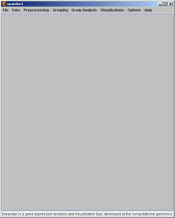
Upon running the program, the main menu bar appears:

Input Data

 

Expander operates on two types of data:

a) Gene Expression data – can be either cDNA microarray data (expected as log 2 (R/G)) values OR Oligonucleotide array data (expected as positive expression levels). If R is installed, oligonucleotide data can also be loaded from a directory containing several .cel files.

If one wishes to perform functional analysis or promoter analysis, an ID conversion file should be loaded along with the data file. The conversion file maps each probe ID (first column) in the data file into a corresponding conventional gene ID that is used in the GO annotation and TF fingerprint files that are supplied with EXPANDER.

b) Gene sets data – contains predefined sets of genes. In this data type, the conventional gene IDs that are used by EXPANDER in the GO annotation and TF fingerprint files are expected.

For details regarding the Gene ID convention that is used for each organism, refer to the Supplied files section.

For details regarding the data files formats see the File Formats section.

 

Loading gene expression data:

To load expression data, select: File >> New Session. From the submenu select Expression Data>>Tabular Data File or .cel Files.

Tabular Data File

When selecting Tabular Data File, the following dialog box will appear:

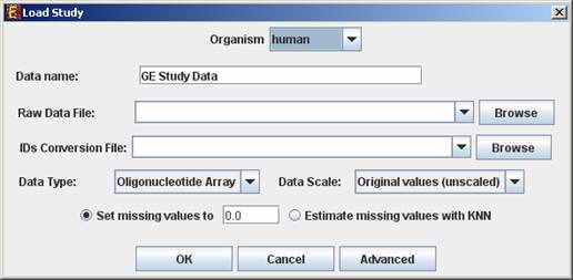
Data type and scale are to be determined according to the input file. If the file contains missing values, these values will be estimated upon loading the data either by setting them to and arbitrary value (if the ‘Set missing value to ____’ option is selected) or by utilizing the KNN (K-Nearest Neighbors) method (if the ‘Estimate missing values with KNN’ option is selected).

Upon pressing the ‘Advanced’ button after filling the ‘Raw Data File’ field, an ‘Advanced dialog box’ appears. This dialog box can be used in order to facilitate the data load of files that are not in the required format. It also enables the user to input a floor value, to which all entries that are below that value will be set (this option is available only for oligonucleotides data). The first few rows and columns of the data are displayed in a table, demonstrating the way the data is read by the program according to the current input values.

 

 

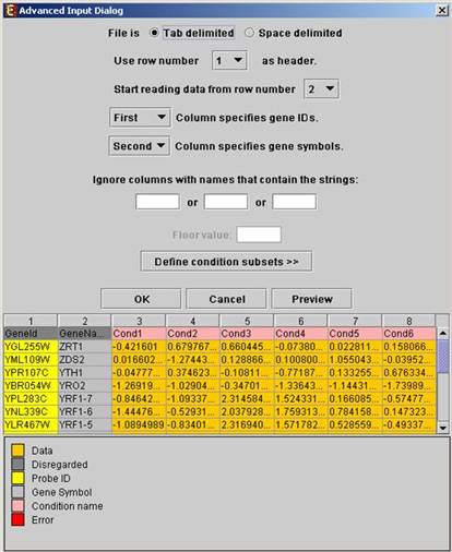
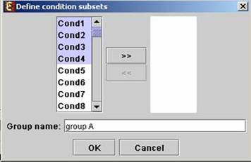
Upon pressing the ‘Define condition subsets’ button, a dialog box appears, enabling the grouping of conditions under a common subset name. This partition is used for visualization purposes.

 

CEL Files

Before loading CEL files, please make sure you have R software along with the Bioconductor “affy” package installed. An open internet connection is also required for this operation.

When selecting .cel Files, the following dialog box will appear:

 

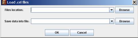
Please browse to the folder where the .cel files are located (Files location), and choose where to save the expression file resulting from the CEL files preprocessing.

If Expander cannot find your R software, a window will pop, asking you to specify its location. Please browse to the location of your R software. In Windows, R.exe file is likely to be located in the 'bin' folder of R software. In Linux, you may type 'which R' in the command line to find R path. If you have a few versions of R installed, please make sure to point Expander to a version in which the Bioconductor “affy” package has been installed.

You may also specify R location from the menu: Options >> Settings >> External applications.

Once the CEL files preprocessing is done, a corresponding tabular data file is generated and a 'Load Study' dialog will appear, as in loading Tabular  Data.

 

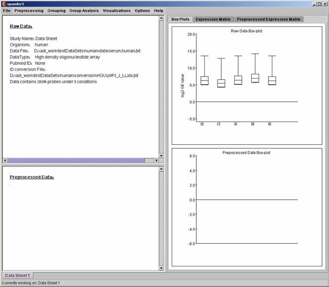
After loading a gene expression data set, a ‘Session Data’ display tab is added to the main window (see example below). It contains information regarding the raw data file, a box plot chart, and an expression matrix visualization of the raw data.

 

 

Loading gene sets data:

To load Gene Sets data select File>>New Session. From the submenu select Gene Sets.

The following dialog box will appear:

 

 

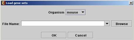
For details regarding the data files formats see the File Formats section.

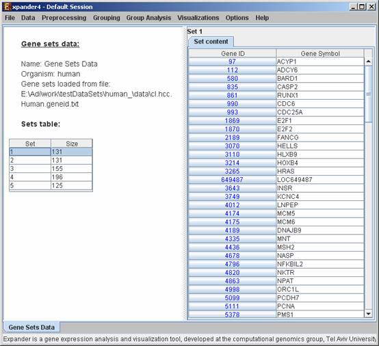
After loading a gene sets data, a ‘Session Data’ display tab is added to the main window (see example below). It contains information regarding the data file, and a table describing the different sets (set number and size). Upon clicking on a row in the table, the corresponding gene list appears on the right.

 

 

 

 

 

Preprocessing GE Data

The following preprocessing schemes can be performed using EXPANDER:

1)     Flooring: setting all expression values that are bellow a certain threshold (set by the user) into that threshold. This can be performed through the ‘Advanced Data Load’ dialog box, and is available only for oligonucleotide data. 

2)     Merging conditions (Preprocessing >> Merge conditions): merging a selected set of condition profiles (columns) in the dataset into one profile, in which each entry holds the average value of the merged entries.

3)     Normalization: required in order to remove systematic variation, i.e. variation arising from reasons other than biological differences between RNA samples. Expander performs normalization only for oligonucleotide data, since it is assumed that the cDNA microarray data is already normalized, as it is input after performing log ratio (log2R/G).

Normalization can be performed using the following schemes:

a)     Quantile normalization (Preprocessing >> Normalization >> Quantile), in which the whole data is used.

b)     Non-linear baseline normalization (Preprocessing >> Normalization >> Non Linear Baseline), which uses a baseline array (can be selected by the user). In this scheme a normalization function is calculated using pseudo Loess regression of the M vs. A scatter plot. The subset of genes that are used to evaluate the normalization function can be set to ‘all genes’ (recommended when most genes in the dataset are expected to be constantly expressed) or a ‘rank invariant set’ of genes (recommended when there can be a large number of differentially expressed genes).

For more details regarding the normalization schemes see the References section.

4)     Condition filtration: the conditions used in the analysis can be manually filtered by selecting: Preprocessing>>Filter Conditions. This will bring up a dialog box in which the user can select the required conditions from a list.

5)     Gene (probe) filtration:  can be performed in order to filter out some of the constantly expressed genes, and perform downstream analysis on a smaller informative subset of the genes.

     Probe filtration can be performed using the following schemes:

a)     t-Test (Preprocessing >> Filter Probes >> t-Test): When using this method, only probes that demonstrate differential expression between two condition subsets are selected.

b)     Fold Change (Preprocessing >> Filter Probes >> Fold Change): when using this method only genes that are over/under expressed by at least n fold in at least k arrays are selected (n and k are determined by the user). The fold change can be calculated in relation to (a) a selected baseline array (b) the minimal expression value of the gene OR (c) the reference value when working on cDNA microarrays (depending on the user’s selection).

c)     Variation (Preprocessing >> Filter Probes >> Variation): In this method, the k most variant genes are selected (k is determined by the user). Variance is used to measure variation for cDNA Microarray data, and Coefficient of Variation is used to measure variation for oligonucleotide data.

 

6)     Standardization: When expression values between different genes are very different, but general expression patterns are similar (high Pearson Correlation values), we would expect to see this similarity when looking on a pattern display. Since the absolute values of expression are different, a manipulation is required, in order to view the patterns on the same scale. This manipulation is called standardization.

     Standardization can be performed using the following schemes:

a)     Mean 0 and Variance 1 (Preprocessing >> Standardization >>Mean 0 and Variance1) – normalizes each expression pattern to have a mean of 0 and a variance of 1. This method is appropriate in most cases when working on genes.

b)     Log data (Preprocessing >> Standardization >> Log Data) – Performs log2 operation on each entry.

c)     Fixed norm - normalizes each expression pattern to have a fixed norm i.e. expression levels are divided by the norm of that expression vector (the root of sum of squares of that vector). This method is appropriate when different mean values or variances are expected for different patterns (e.g. when working on conditions and expecting larger variance in later phases of a response.

After performing a preprocessing operation, the information regarding the operation is added to the ‘Preprocessed Data’ section in the ‘Session Data’ tab. In addition, the ‘Preprocessed Data box plot’ and ‘Preprocessed Expression Matrix’ are automatically updated according to the new values in the data.  

 

 

 

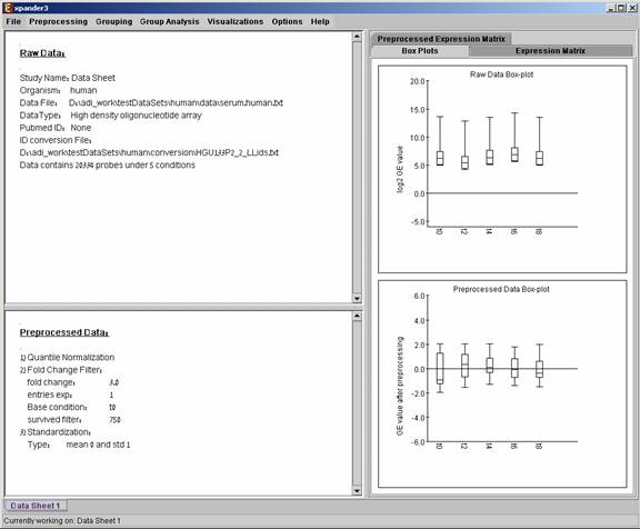
Upon selecting Preprocessing >> Undo the data is changed to be as it was before the most recent preprocessing operation was performed, and the corresponding information is removed from the ‘Preprocessed Data’ section. The ‘Preprocessed Data box plot’ and ‘Preprocessed Expression Matrix’ are automatically updated accordingly.

All the above operations can be performed before running further analysis on the data and generating displays.  When attempting to perform further preprocessing operations after analysis results and visualizations have been generated, the following dialog box appears:

 

 

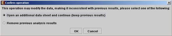
Upon choosing to open an additional data sheet, a new data set view tab called ‘Data Sheet 2’ is added to the main frame. The title of this tab is highlighted (colored in purple), indicating that it is now the active data sheet (i.e. all further operations refer to this data sheet). The active data sheet is automatically changed according to the selected (front) visualization tab.

Preprocessed gene expression data can be saved to a file at any time be selecting Preprocessing >> Save Preprocessed Data. The data is written in the same format defined for input GE data.

 

Viewing Data Plots

 

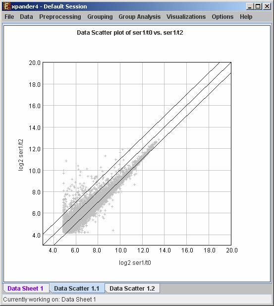
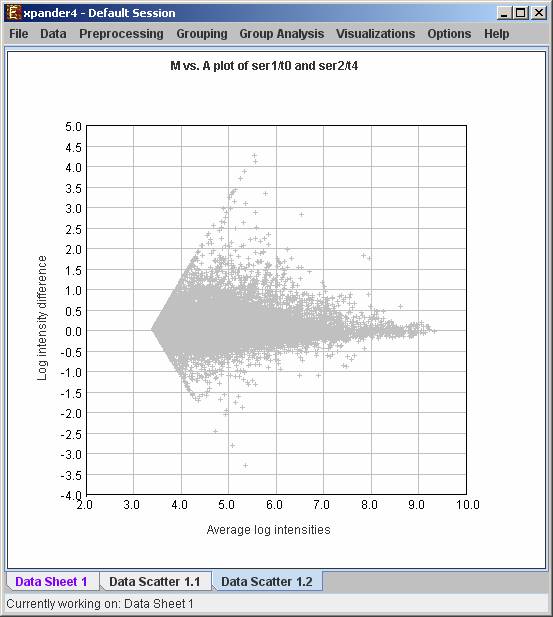
Expander provides two types of scatter plots visualizations that can be operated via Preprocessing >> Normalization >> View Scatter Plots.

 

Simple plot - Displays a scatter plot of two arrays (selected by the user), in which the ith point (xi,yi) represents the expression value (log expression for oligonucleotide data) of the i^th gene in one array vs. the other. For normalized data, points should be located around the y=x line (marked on the scatter plot).

 

 

M vs. A plot (available only for oligonucleotide data) - Displays a scatter plot in which each point (Ai,Mi) represents the log intensity difference of the i th probe in the two arrays (selected by the user) vs. the average log value of these intensities.

  

 

 

Clustering GE Data

 

The goal of clustering is to partition the genes into distinct sets such that genes that are assigned to the same cluster should have similar expression patterns, while genes assigned to different clusters should have non-similar expression patterns.
Usually there is no one solution that is the ‘true’ mathematical solution for this problem, but a good clustering solution should have two merits:

(1)   High homogeneity (average similarity between genes from the same cluster).

(2)   High separation (average distance/dissimilarity between genes from different clusters).

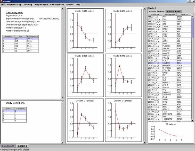
After operating one of the clustering algorithms a clustering results view appears. The view contains information about the solution and its quality including the method and parameters that were used to obtain it, number of clusters, number of singletons (probes that were not assigned to any cluster), overall homogeneity and separation, as well as the size and homogeneity of each cluster. This summary can be used to compare different solutions. 

In order to apply a clustering algorithm to the data, select the required algorithm from the Grouping >> Clustering menu (options are: KMeans, CLICK, SOM). You can also load an existing clustering solution from a file by selecting the Load Solution option from the Clustering menu (For details regarding the clustering solution file format, refer to the Files Format section).

The CLICK algorithm is not designed to find clusters under the size of 15 probes, so it might fail in clustering small datasets.

Fill the required input data in the algorithm input dialog box and press the ‘Ok’ button.
The parameters required for each method are as follows:

 

Details about the algorithms can be obtained through the relevant articles in the References section.

After clustering is performed, a clustering solution visualization tab is added to the main window. It contains the following views:

Information regarding the clustering algorithm, number of clusters, number of un-clustered elements (singletons), and numerical measures of the clustering quality, including:

a)     Overall average homogeneity - calculated as the average value of similarity between each element and the center of the cluster to which it has been assigned, weighted according to the size of the cluster.

b)     Overall average separation – calculated as the average similarity between mean patterns of different clusters, weighted according to their sizes.

c)     Clusters table - contains the number, size and homogeneity of each cluster. 

Mean Patterns of all clusters with error bars (±1 STD).

A table listing all condition titles and their corresponding number used in the patterns display. Upon selecting a row in this table, the corresponding column in each of the mean pattern plots is marked.

Upon selecting a cluster (from the clusters table or from the mean patterns view), the corresponding probe list, probe patterns and expression matrix are displayed on the right.

 

 

After performing Promoter analysis or Functional analysis (for details see the Group analysis tools section), if the selected cluster has been found to be enriched with TF binding sites or GO annotations, the corresponding histogram and analysis information are added to the single cluster view.

A clustering solution can be saved using the Grouping >> Clustering >> Save Solution, and reloaded using the Grouping >> Clustering >> Load Solution.

 

Biclustering GE Data

 

Biclustering is clustering of both genes and conditions of the data into subgroups that are not necessarily disjoint. It enables the user to detect genes that are co-regulated in only a subgroup of the conditions, and does not force genes to belong exclusively to one cluster. It is useful when working on datasets which contain a large number of conditions.

Biclustering is performed by Expander using the SAMBA algorithm (for details see the References section).

In order to apply the SAMBA biclustering algorithm to the data select Grouping>>Bi-Clustering>>SAMBA. The following dialog box will appear:

 

 

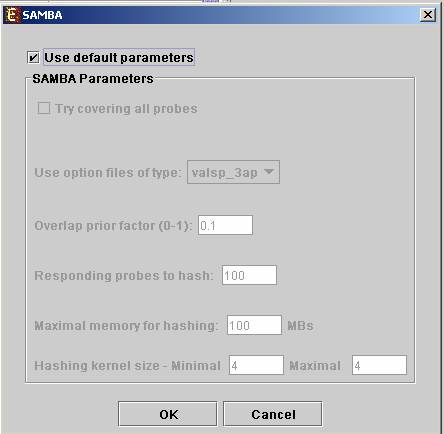
It enables the configuration of some of the parameters for the algorithm. The following table specifies the different parameters that can be set via this dialog box:

 

 

Upon clicking ‘OK’ in the dialog box, the SAMBA algorithm is operated on the dataset.

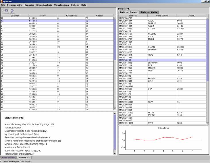
After biclustering is performed a biclustering solution visualization tab is added to the main window. It contains the following views:

a)     Information regarding the biclustering algorithm, and number of resulting biclusters.

b)     Biclusters table – contains the following information for each bicluster: serial number, score, number of probes genes and number of conditions. The score is given by the SAMBA algorithm and is size-dependent, thus, it is not recommended to use it to compare the quality of two biclusters of different sizes. The table can be filtered to display a subset of the biclusters by clicking on the ‘Filter’ () button in the toolbar. Filtering can be performed according to: Score, number of probes and number of conditions.

Upon selecting a bicluster (from the biclusters table), the corresponding probe list, probe patterns and expression matrix are displayed on the right.

 

 

 

 

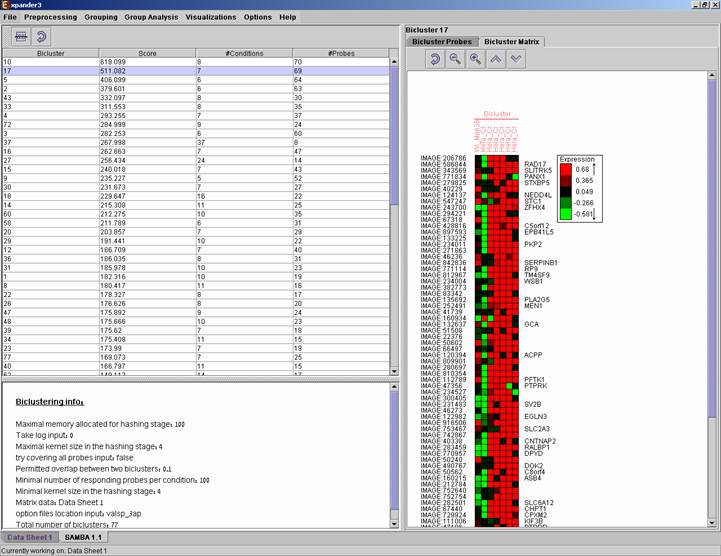
After performing Promoter analysis or Functional analysis (for details see the Group analysis tools section), if the selected bicluster has been found to be enriched with TF binding sites or GO annotations, the corresponding histogram and analysis information are added to the single bicluster view, and a column is added to the expression matrix display for each enrichment class, stating for each probe, whether it belongs to that class.

A biclustering solution can be saved using the Grouping >> Bi-Clustering >> Save Solution, and reloaded using the Grouping >> Bi-Clustering >> Load Solution. For a format of the solution file, please refer to the File Formats section:

Group analysis tools

 

The following analysis can be performed on gene sets, clusters, biclusters, or the filtered dataset (the analyzed set of probes as one set).

 

Functional Analysis:

This tool performs basic statistical analysis on the distribution of functions of genes within each cluster. The functions of the genes are determined according to annotation files (GO), which can be downloaded from the EXPANDER download page (see the Supplied Files section). To perform this analysis, Expander utilizes the TANGO software, which performs hyper-geometric enrichment tests and corrects for multiple testing by bootstrapping and estimating the empirical p-value distribution for the evaluated sets. 

Before operating functional analysis the annotation files for the relevant organism should be downloaded from the download page. To perform the analysis, select Group Analysis >> Functional Analysis >> TANGO. The following dialog box will appear: 

 

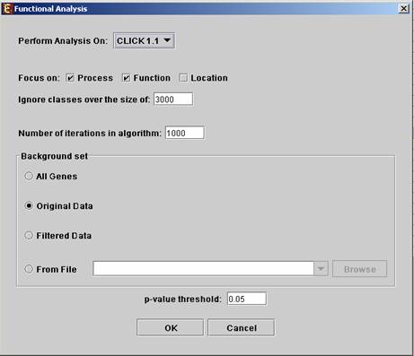
The following table specifies the different parameters that can be set via this dialog box:
 

 

Upon clicking ‘OK’ in the dialog box, the TANGO algorithm is operated.

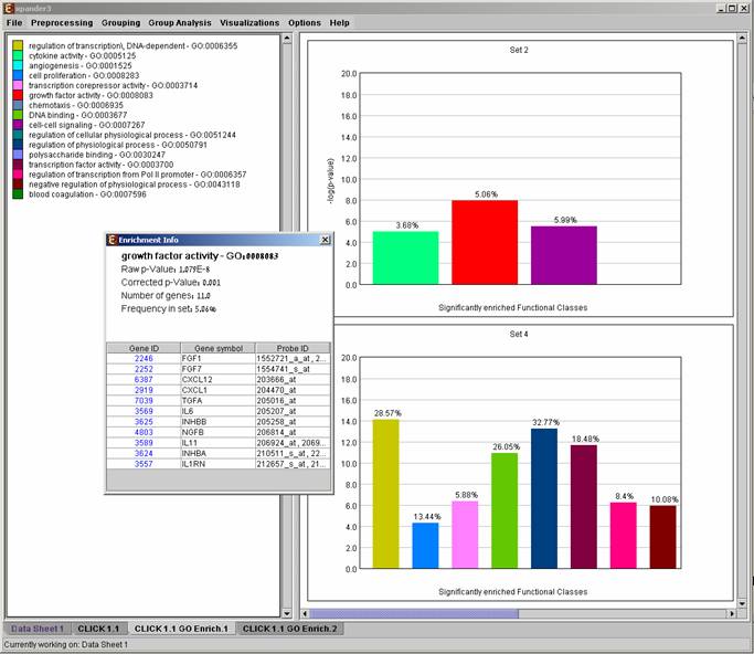
After functional analysis is performed a functional analysis solution visualization tab is added to the main window. The results are displayed using a histogram for each cluster/bi-cluster in which enrichment has been detected. Each histogram contains a column for each significant (more frequent than would be expected by random) functional class. The definition of significant depends on the user’s selection of threshold p-value i.e., a functional class is considered significantly enriched in a cluster/bicluster if its corrected p-value is lower than the preset threshold p-value.

The height of the column is proportional to the significance of this enrichment (i.e. height = -log(raw p-value)). The frequency in set (frequency of binding site within the examined set, in %) of the class in the cluster is written on top of the column.  Upon clicking on a column, a dialog box is displayed containing the class name, raw p-value, corrected p-value, and a list of the genes in the cluster/bi-cluster that belong to the class. Upon clicking on one of the gene Ids in the table, a relevant web page with information regarding this gene is displayed. The display tool tip shows the cluster number, size and homogeneity.

 

 

Annotation files are currently supplied with EXPANDER for yeast, human, mouse, rat, fly, zebrafish, c-elegans, arabidopsis and chicken, and are updated on a regular basis (for more information, refer to the Supplied Files section).

The results of this analysis can be exported to a text file (using the display menu item Group Analysis>>Functional Analysis>> Export Results). The format of the produced text file is as follows:

Cluster: <cluster number>, size: <cluster size>

<enriched functional class 1>
=================
p-value  = <p-value>

<gene Id>; <gene symbol>; <probe1 id>, <probe2 id>...
<gene Id>; <gene symbol>; <probe1 id>, <probe2 id>...
…
<enriched functional class 2>
=================
p-value  = <p-value>

<gene Id>; <gene symbol>; <probe1 id>, <probe2 id>...
<gene Id>; <gene symbol>; <probe1 id>, <probe2 id>...
.
.
.
etc.

 

Promoter Analysis:

This tool identifies TFs whose binding sites are significantly over-represented in a given set of promoters (i.e. cluster or bicluster). To perform this analysis Expander utilizes the PRIMA (PRomoter Integration in Microarray Analysis) software which performs a statistical analysis on the distribution of transcription factor motifs in the promoters of genes within each cluster or bicluster. To achieve this, PRIMA uses preprocessed TF fingerprint files, which can be downloaded from the EXPANDER download-page (see the Supplied Files section), and are updated on a regular basis.  For details regarding the PRIMA software see the References section.

Before operating promoter analysis, the TF fingerprint file for the relevant organism should be downloaded from the download page. To perform the analysis, select Group Analysis >> Promoter Analysis >> PRIMA. The following dialog box will appear:

 

 

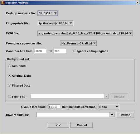
The following table specifies the different parameters that can be set via this dialog box:

 

 

 

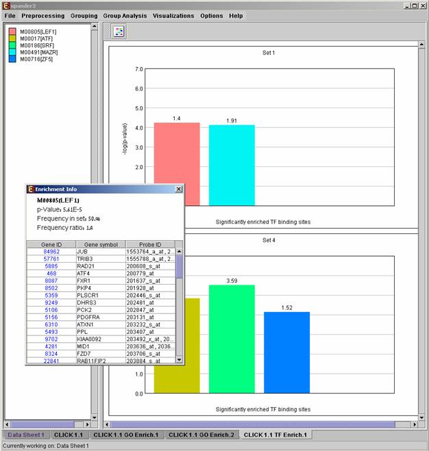
After promoter analysis is performed, a promoter analysis solution visualization tab is added to the main window. The results are displayed using a histogram for each probe set (cluster/bi-cluster) in which enrichment has been detected. Each histogram contains a column for each significant (more frequent than would be expected by random) TF binding site. The definition of significant depends on the user’s selection of threshold p-value. i.e., a TF binding site is considered significantly enriched in a cluster/bicluster if its corrected p-value is lower than the preset threshold p-value.

The height of a column is proportional to the significance of this enrichment (i.e. height = -log(p-value)), and the frequency ratio (in %) of the class in the cluster vs. the background set is written on top of the column. Upon clicking on a column, a dialog box is displayed containing:

TF accession number in TRANSFAC DB [TF name], p-value, % of covered promoters in cluster, relative frequency (frequency in cluster divided by frequency in background set) and a list of the genes in the cluster which contain the motif in their promoters. Upon clicking on one of the gene Ids in the table, a relevant web page with information regarding this gene is displayed. The display tool tip shows the cluster number, size and homogeneity.

 

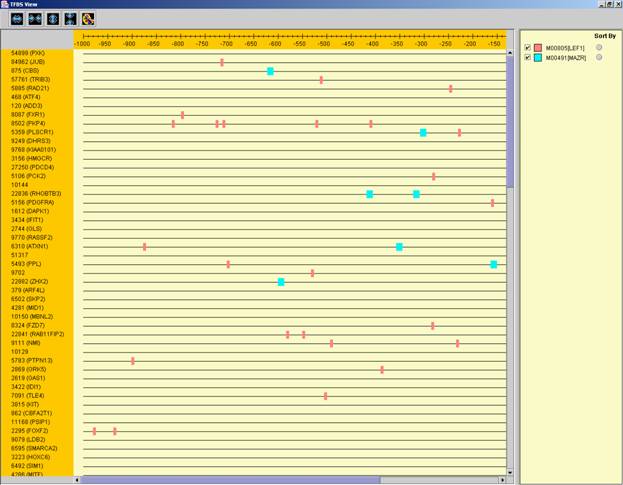
After performing promoter analysis, TF binding sites can be viewed by selecting Group Analysis >> Promoter Analysis >> View Binding Sites OR by pressing the toolbar button (). After selecting the set (cluster/bi-cluster) to be viewed, a separate frame is displayed, containing a line to represent each of the genes in the set, and a colored rectangle, to represent each binding site. A color index appears on the right, mapping each color to the corresponding TF (PWM). A check box next to each of the entries in the color index allows hiding any of the PWMs, and a radio button next to each of the entries in the color index allows sorting the genes in the display according to the number of hits of the corresponding TF. The toolbar contains tools for vertical and horizontal zooming. If a sequence file had been selected via the promoter analysis input dialog, the actual sequence will be displayed when the zoom factor (scale) allows it.

 

TF motif fingerprint files and promoter sequence files are currently supplied with EXPANDER for yeast, human, mouse, rat, fly, zebrafish, c-elegans, arabidopsis and chicken, and are updated on a regular basis (for more information, refer to the Supplied Files section).

The results of this analysis can be exported to a text file (using the display menu item Group Analysis >> Functional Analysis >> Export Results). The format of the produced text file is as follows:

Cluster: <cluster number>, size: <cluster size>

<enriched PWM1 name>
=================
p-value  = <p-value>

<gene Id>; <gene symbol>; <probe1 id>, <probe2 id>...
<gene Id>; <gene symbol>; <probe1 id>, <probe2 id>...
…
<enriched PWM2 name>
=================
p-value  = <p-value>

<gene Id>; <gene symbol>; <probe1 id>, <probe2 id>...
<gene Id>; <gene symbol>; <probe1 id>, <probe2 id>...
…
etc.

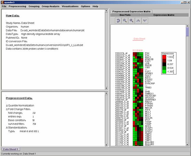
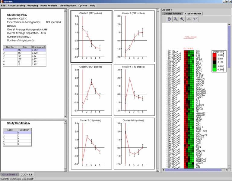
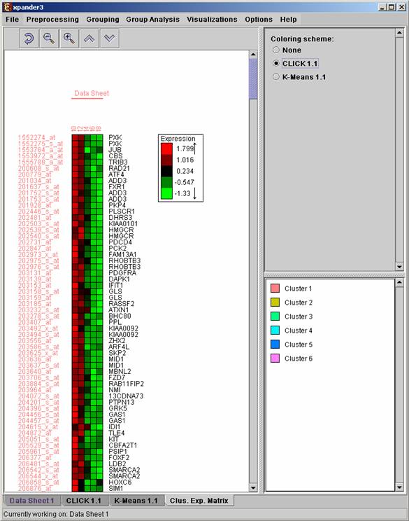
 Matrix visualizations

 

An expression matrix visualization is integrated in many of EXPANDER’s displays. This visualization is similar to the red-green matrix representation of Eisen et al (1998).  All it does is to render the gene-expression data on the screen in color, where green indicates under expression, and red indicates over expression. Color rendering can be configured by the user in one of the following manners: (a) by setting the range (top and bottom values) of rendered values (default values are set according to the data scale, e.g. 40-1000 for non-standardized oligonucleotide data) or (b) by setting the percent of values, which are to be disregarded as extreme values from each edge (by default set to 5%). The manner of color scale configuration (i.e. (a) vs. (b)) can be set via the ‘Data Matrix View’ tab in the ‘Display Settings’ dialog box, available from Options >> Settings.

A color scale appears next to the matrix (upper right side). The displayed tool tip shows the probe ID and condition title corresponding to the row and column on which the cursor is placed, and the expression value in that position. The matrix toolbar contains zoom in, zoom out, reset scale (to reset zoom factor), shorten condition title and Elongate condition title tools. 

Upon selecting Visualizations >> Clustered Expression Matrix, a clustered expression matrix visualization tab is added to the main window. The probes are ordered in their original order. If a clustering solution has been previously created, its’ name appears next to a radio button in the top right panel. Upon pressing this button, the order of the probes in the display changes and probe IDs are colored according to the clusters. The color index at the bottom right panel, maps each color to the index of the corresponding cluster.  

 

 

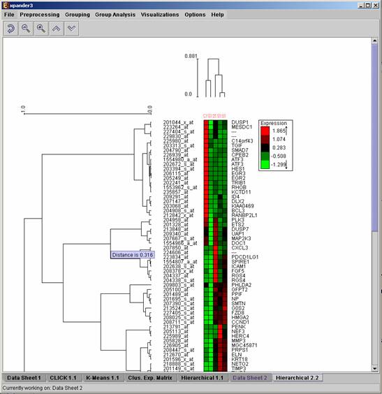
Hierarchical clustering and visualization

 

This tool uses the agglomerative algorithm to calculate a dendrogram tree for all expression patterns (probe patterns) and/or profiles (condition profiles). The type of linkage (manner in which the distance between a new node and the rest of the nodes is calculated) used in the algorithm can be set via an input dialog (for details regarding the algorithms refer to the References section). Note that it does not generate a partition of the probes to clusters. The distance measurement used in the algorithm is (1-Pearson Correlation)/2.

To perform hierarchical clustering, select Grouping >> Hierarchical Clustering. Upon selecting this option, a dialog box appears in which the ‘linkage type’ parameter, used in the algorithm can be set. After pressing ‘OK’, the algorithm will be operated both on the probe patterns and on the condition profiles.

The resulting trees are displayed next to an expression matrix so that the probe tree appears vertically on the left and the condition tree appears horizontally above the matrix. The scale next to each tree indicates the range of distance values between vectors corresponding to the leaves. The tool tip indicates the distance value corresponding to the cursor location on the tree.

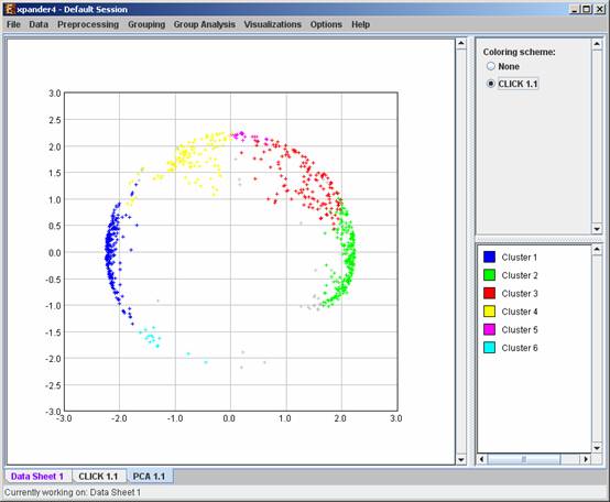
PCA transformation

This tool transforms the original data from a k (original pattern length) to a 2 dimensional space, so that each expression vector is represented by a dot on an XY scatter chart. The transformation is based on the PCA (Principal Component Analysis) algorithm. To operate the tool, select Visualizations >> PCA.

If a clustering solution has been previously created, its’ name appears next to a radio button in the top right panel. Upon pressing this button, the color of each dot in the display changes according to the cluster assignment of the corresponding probe. The color index at the bottom right panel, maps each color to the index of the corresponding cluster.

 

Additional options

 

Saving and loading sessions

A set of analysis operations performed on one data set can be saved by selecting File >> Save Session. It can later be reloaded by selecting File >> Load Session. Loading a previously saved session will bring up all analysis output and visualizations that had been generated in that session, and the user will be able to continue working where he had previously stopped.

 

Closing views

The user can close all open views by selecting File >> Close All.

Closing a single view can be performed either by selecting File>>Close when the relevant view is selected OR by right clicking on the tab title of the relevant view and selecting Close from the popup menu.

 

Docking a view into a separate frame

Can be performed either by selecting Options >> Dock into external frame when the relevant view is selected OR by right clicking on the tab title of the relevant view and selecting Dock into external frame from the popup menu.

Upon creating the separate frame, the view will be removed from the main window. Upon closing the separate frame generated in this manner, the view will be retrieved into the main window.

 

Accessing the EXPANDER download page

The Expander download page can be accessed directly by selecting Help >> Open Download Page, while the machine is connected to the Internet.

 

Printing the display

Each display can be printed by selecting File >> Print while its tab is selected.

 

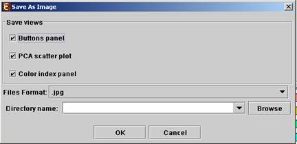
Exporting display into image files

Each display can be exported into image files of type .jpg, .png or .eps (post-script). This can be done by selecting File >> Save As Image. Upon selecting this option, a dialog box, similar to the following is displayed. In the dialog box the saved images (sections of the view), image files format, and destination directory name are input.

 

 

 

File Formats

Expression data file format:

1) Suffix: no limitations. 
2) Separating token: tab delimiter.
3) Format:

1st line: contains the string ‘probeId’ and a tab delimiter, followed by the string ‘geneSymbol’ and a tab delimiter, followed by the names of all conditions separated by tab delimiters.

Next lines: Each subsequent line consists of the probe ID (an identifier string that is unique to each probe in the chip), followed by a string, which represents the gene full name (if missing can be left empty by adding an additional tab delimiter), followed by its expression values (all tab delimited). If the expression file contains missing values, Expander either replaces them with a preset value (0 by default), or estimates them using the KNN (K-Nearest Neighbors) method, depending on the user selection in the data load dialog box.

*For example see files ‘expressionData1.txt’ and ‘expressionData2.txt’ in the Expander/sample_input_files/ directory.

If the data is not in the above format, it may be possible to load it using the ‘Advanced’ dialog box, which appears upon pressing the ‘Advanced’ button in the Expression Data load dialog box (see Loading Input Data).

 

Gene Sets file format:

1) Suffix: no limitations

2) Format: Each line contains a gene ID, a gene symbol (optional, can be configured in the 'Advanced' dialog box) and the number of its set (separated by tabs). The gene IDs are expected to be of the same convention used in the GO annotation and TF fingerprint files.  For details regarding the Gene ID convention that is used for each organism, refer to the Supplied files section.

*For example see file ‘geneSetsData1.txt’ under the Expander/sample_input_files/ directory (see Sample input files for more details).

 

ID conversion file format:

1) Suffix: Currently, there are no limitations regarding the file name suffix.

2) Format: Each line contains the probe id as it appears in the data file, a tab separator and the corresponding gene ID (e.g. Entrez/Locus-Link ids for mouse and human genes and ORF codes for yeast).  The second field can be left blank, indicating no conversion for that probe ID.

* It is possible that several probe IDs in the data file will be mapped to the same gene ID (e.g.: several ESTs from the same gene).

 

Clustering files format:

1) Suffix: no limitations.

2) Format: Each line contains the probeID, a tab separator and the number of its cluster.
Cluster number 0 is reserved for genes that are left unclustered. The file does not have to contain all genes in the data. If a gene does not appear in the file, it is automatically set as unclustered.  

*For example see file ‘expressionData1Clustering.sol’ (a clustering solution for the data file’ expressionData1.txt’) under the Expander/sample_input_files/ directory (see Sample input files section for more details).

 

Biclustering files format:

1) Suffix: `.bic`.
2) Format: the file is composed of two parts, presented here.

Part 1 presents a summery of the biclusters found.

• It begins with the string: `[Bick]` in the first line.
• Following lines contain the bicluster's id followed by its' score, separated by a tab delimiter (a line for each bicluster).

Part 2 presents the probesets and the conditions contained in each bicluster.

• It begins with the string: `[Bicd]` in the first line.
• Following lines contain the bicluster id, type of element ('0' for condition, '1' for probe) and element id (name of condition or probe ID), separated by tab delimiters.

 

Background set files format:

1) Suffix: no limitation.

2) Format: each line should contain one gene ID. The gene IDs are expected to be of the same convention used in the annotation and TF fingerprint files for the organism you are working on (please refer to the Supplied files section).

 

Sample input files

 

Several sample files are provided under Expander/sample_input_files/. These files include:

expressionData1.txt – A gene expression data file that was generated using the cDNA microarray technology. This is a partial dataset extracted from a yeast cell cycle dataset generated by Spellman et al 1998 (see the References section). Gene identifiers in this set are yeast ORFs, which are the same identifiers used in the annotation and TF fingerprint files that are supplied with Expander. Thus, no conversion file is required.

expressionData2.txt – A gene expression data file that was generated in the Affymetrix technology. This dataset was generated in an experiment that was conducted in out laboratory on human cells, and has not yet been published. Affymetrix chips of type HG-Focus were used for this experiment and thus, the HG-Focus conversion file is required for the analysis (can be downloaded from the download page).

expressionData3.txt – taken from Murray JI, Whitfield ML, Trinklein ND, Myers RM, Brown PO, Botstein D: Diverse and specific gene expression responses to stresses in cultured human cells. Mol Biol Cell 2004, 15:2361-2374. A corresponding conversion file (from clone-IDs to LL-IDs) is available at the same directory under the name Data3Conversion.txt.

expressionData1Clustering.sol – A clustering solution that was generated by Expander for the dataset in ‘expressionData1.txt’.

geneSetsData1.txt - Contains sets of human genes (in Entrez/Locus-Link IDs).

 

Supplied Files

 

Annotation and TF-fingerprint files

Annotation and TF-fingerprint files are currently supplied with Expander for yeast, human, mouse, rat, fly, zebrafish and c-elegans and are updated on a regular basis.

The following conventional gene IDs are used in the annotation and TF-fingerprint files:

 

 

Gene ontology and annotation files

The gene ontology and annotation files supplied with Expander are based on data that was downloaded from the GO website.

The following table specifies the database from which these files are derived for each of the organisms that we support, and the date of download from GO site: 

 

 

 

 

 

 

 

 

 

 

 

 

 

 

 

 

 

 

 

TF fingerprint files and sequence files

The following TF fingerprint files (and sequence files) can be downloaded from our web download page (as part of the zip supplied for each organism).

 

 

 

 

Gene ID conversion files:

Gene ID conversion files for many of the Affymetrix chips can be downloaded from the Expander download page. The files map each Affy Id into the corresponding Entrez/LocusLink Id. Conversion files are generated and added to the download page according to user requests.

 

 

 

 

Settings

The Settings are accessible from the Options menu, and contain Display settings External applications settings.

 

The Display dialog box contains the following tabs:

Clustering Results View – Contains a check box that configures whether the Y-axis scale of all cluster patterns is common OR cluster specific.

Group Analysis Results View – Contains a check box that configures whether the Y-axis scale of all histograms is common OR cluster specific.

Data Matrix View – Allows selection between range control and extreme values control when rendering expression matrix values.

 

The External applications dialog box allows specification of the location of the R executable (required for CEL files loading). In Windows, R.exe file is likely to be located in the 'bin' folder of R software. In Linux, you may type 'which R' in the command line to find R path.

                      

 

 

 

 

FAQ

 

Linux/Unix problems

Click clustering, Samba bi-clustering and Prima Promoter analysis algorithms fail when running on Linux/Unix.

 

CEL Files Loading Problems

How do I install R and the Bioconductor "affy" package?

Loading of CEL files fail.

 

Clustering

When I try to run Biclustering on my data I get a failure notice.

How can I save the clustering expression patterns charts?

 

Grouping Analysis (functional and promoter analysis)

When I run Functional Analysis, Expander gets stuck.

When I load a session with that contains Functional Analysis results, Expander gets stuck,

When I try to run Promoter Analysis no values appear in the Fingerprints file field of the input dialog box.

When I try to run the promoter\functional analysis, I get a failure message box.

Promoter\Functional analysis produce no results (the resulting view is empty).

How can I save the bar charts produced by Expander, displaying the enrichments?

Why do certain Transcription Factors have a few accession numbers or\and a few gene IDs?

 

 

Click clustering, Samba bi-clustering and Prima Promoter analysis algorithms fail when running on Linux/Unix.

Answer: Make sure that you have write permission in the Expander directory, and execution permissions on the files: click.exe, samba.exe and analyzeFingerprints.exe, which are under the Expander directory. If the problem still occurs, open the file expanderLog.txt and search for the text: “libstdc++.so.5”. If this text appears (along with a message indicating it has not been found), please contact your system administrator and report this problem (this is a system problem). If you do not have a system administrator, and fail to install this library, please contact us (expander@cs.tau.ac.il) and we will try to assist.

 

How do I install R and the Bioconductor "affy" package?

Answer: The newly added .cel file preprocessing utility also requires the pre-installation of one of the recent versions of R (can be installed from: http://cran.r-project.org/).  After installing R, please do the following to install the Bioconductor “affy” package:

5)     Run R.

6)     In the R frame\window type the text: source("http://bioconductor.org/biocLite.R")

7)     Press ‘Enter’.

8)     In the R frame\window type the text:  biocLite("affy")

 

Loading of CEL files fail.

Answer: If you are working with Expander version 4, please update to 4.0.1 or higher. Make sure you have R along with the Bioconductor “affy” package installed in the R version which is specified in the settings “External  Applications” tab (from the menu select Options >> Settings >> External applications). If R location is not defined in the settings, please define it (In Windows, R.exe file is likely to be located in the 'bin' folder of R software. In Linux, you may type 'which R' in the command line to find R path). If loading of CEL files still fails, please make sure that the Files location which you specified in the 'Load .cel Files' dialog box, is a folder which contains .cel files and that you have a write permission to that folder.

 

When I try to run Biclustering on my data I get a failure notice.

Answer: Make sure that the ‘Use option files of type’ field in the SAMBA input dialog box is not empty (if it is, please re-download Expander). Also make sure that the following files exist in your Expander directory: ibic.opt, samba.exe.

 

How can I save the clustering expression patterns charts?

When the clustering results tab is open, please go to File >> Save As Image.

 

When I run Functional Analysis, Expander gets stuck.

Answer: If you are working with Expander version 4.0 or 4.0.1, please update to a higher version (4.0.2 and on).

 

When I load a session with that contains Functional Analysis results, Expander gets stuck.

Answer: If you are working with Expander version 4.0 or 4.0.1 (and the session was created with a version < 4.0), please update to a higher version (4.0.2 and on).

 

When I try to run Promoter Analysis no values appear in the Fingerprints file field of the input dialog box.

Answer: Fingerprint files are not placed in the right directory. Fingerprint files should be placed under the ‘TF_fingerprints’ directory that is under the Expander/organism/<org name> directory. For example, the human FP file should be placed under: …/Expander/organisms/human/TF_fingerprints/. When downloading the organism specific data zip, it should be extracted into the Expander/organisms/ directory. This will automatically put them in the right place.

 

When I try to run the promoter\functional analysis, I get a failure message box.

Answer: Errors while running promoter\functional analysis can be caused by the following problems:

a)  Organism specific data (Fingerprint\annotation files) is not in the right directory. The organism specific data zip should be extracted into the Expander/organisms/ directory.

b)   Data contains elements that do not appear in the background set (this is only relevant when the background set is loaded from an external file).

 

Promoter\Functional analysis produce no results (the resulting view is empty).

Answer: This can be caused by one of the following:

a) You are using the wrone conversion file or a conversion file that is not in the right format or does not map the probes to the expected type of gene Ids. The conversion file maps each probe ID in your data file to a gene ID that is used in the promoter and functional analysis. It is requires if the probe Ids that you are using in your data file do not match the ones in the annotation and TF_fingerprint we supply.

b) You did not set the organism field in the input dialog to the organism type of your data.

c) You are trying to analyzed only one set (e.g. the filtered data set) which you are using also as background (in this case the analysis has no meaning since it is trying to detect enrichments in the cluster/bicluster in comparison to the background set).

d) You set the threshold p-value to be too strict (low).

e) Biological reason i.e., there is nothing to report regarding this specific clustering/biclustering solution or this gene sets data.

 

How can I save the bar charts produced by Expander, displaying the enrichments?

When the results tab is open, please go to File >> Save As Image.

 

Why do certain Transcription Factors have a few accession numbers or\and a few gene IDs?

Answer: The transcription factors (TFs) found enriched by Prima are presented in the following way:

Accession Num. in TRANSFAC DB [TF name]. For example, M00287[NF-Y]

It is possible that a TF will have a few accession numbers in TRANSFAC, which represent different PWMs (position weight matrices specify the probability for observing each nucleotide at each position of the binding site, based on a set of empirically validated binding sites of the respective TF).

It is also possible that a TF will have a few Entrez gene IDs, since a TF may be composed of a few proteins. For example, NF-Y is a trimer, composed of 3 subunits.

 

This section will be updated as we get user feedbacks and problems.

Please refer all questions/comments to Expander@cs.tau.ac.il.

 

 

Copyrights information

Copyrights © Tel-Aviv University, Israel (2003).

This product uses the FreeHEP Java Library, which is distributed under the LGPL license. FreeHEP copyright holders: CERN, Geneva, Switzerland SLAC, Stanford, California, U.S.A. University of California Santa Cruz, U.S.A.

A portion of the user interface code is due to Sun Microsystems.Inc.  Copyright 1994-2004 Sun Microsystems, Inc. All Rights Reserved. The following license rules apply to that portion:

‘Neither the name of Sun Microsystems, Inc. or the names of contributors may be used to endorse or promote products derived from this software without specific prior written permission.

This software is provided ‘AS IS,’ without a warranty of any kind. ALL EXPRESS OR IMPLIED CONDITIONS, REPRESENTATIONS AND WARRANTIES, INCLUDING ANY IMPLIED WARRANTY OF MERCHANTABILITY, FITNESS FOR A PARTICULAR PURPOSE OR NON-INFRINGEMENT, ARE HEREBY EXCLUDED. SUN MICROSYSTEMS, INC. (‘SUN’) AND ITS LICENSORS SHALL NOT BE LIABLE FOR ANY DAMAGES SUFFERED BY LICENSEE AS A RESULT OF USING, MODIFYING OR DISTRIBUTING THIS SOFTWARE OR ITS DERIVATIVES. IN NO EVENT WILL SUN OR ITS LICENSORS BE LIABLE FOR ANY LOST REVENUE, PROFIT OR DATA, OR FOR DIRECT, INDIRECT, SPECIAL, CONSEQUENTIAL, INCIDENTAL OR PUNITIVE DAMAGES, HOWEVER CAUSED AND REGARDLESS OF THE THEORY OF LIABILITY, ARISING OUT OF THE USE OF OR INABILITY TO USE THIS SOFTWARE, EVEN IF SUN HAS BEEN ADVISED OF THE POSSIBILITY OF SUCH DAMAGES.

You acknowledge that this software is not designed, licensed or intended
for use in the design, construction, operation or maintenance of any
nuclear facility.’ 

 

References

Quantile normalization: Bolstad, B. M. Irizarry, R. A.  Astrand, M. and Speed, T. P.  A Comparison of Normalization Methods for High Density Oligonucleotide Array Data Based on Variance and Bias. Bioinformatics   19(2):185-193, 2003. 

Non-linear baseline normalization: Schadt, E., C. Li, B. Eliss, and W. H. Wong. Feature extraction and normalization algorithms for high-density oligonucleotide gene expression array data.  J. Cell. Biochem. 84(S37),120–125, 2002. 

K-Means clustering algorithm: Tavazoie, S., Hughes, J. D., Campbell, M. J., Cho, R. J., and Church, G. M. Systematic determination of genetic network architecture. Nat Genet, 22: 281-285, 1999.

SOM clustering algorithm: Tamayo, P., Slonim, D., Mesirov, J., Zhu, Q., Kitareewan, S., Dmitrovsky, E., Lander, E. S., and Golub, T. R. Interpreting patterns of gene expression with self-organizing maps: methods and application to hematopoietic differentiation. Proc Natl Acad Sci U S A, 96, 2907-2912, 1999.

CLICK clustering algorithm: Sharan, R. and Shamir, R. CLICK: a clustering algorithm with applications to gene expression analysis. Proc Int Conf Intell Syst Mol Biol 8, 307-16, 2000.

SAMBA biclustering algorithm: Tanay, A. Sharan, R. and Shamir, R. Discovering statistically significant biclusters in gene expression data. Bioinformatics, 18(1), 136-144, 2002.

PRIMA algorithm: Elkon, R., Linhart, C. Sharan, R. Samir, R. and Shiloh, Y. Genome-Wide In Silico Identification of Transcriptional Regulators Controlling the Cell Cycle in Human Cells. Genome Research, Vol. 13(5), pp. 773-780, 2003. 

Agglomerative algorithm for hierarchical clustering: Eisen, M. B., Spellman, P. T. et al. Cluster analysis and display of genome-wide expression patterns. Proc Natl Acad Sci U S A 95(25), 14863-8, 1998.

TF binding site profiles that were used to generate the supplied yeast TF fingerprint files: Harbison, C.T., D.B. Gordon, T.I. Lee, N.J. Rinaldi, K.D. Macisaac, T.W. Danford, N.M. Hannett, J.B. Tagne, D.B. Reynolds, J. Yoo, E.G. Jennings, J. Zeitlinger, D.K. Pokholok, M. Kellis, P.A. Rolfe, K.T. Takusagawa, E.S. Lander, D.K. Gifford, E. Fraenkel, and R.A. Young. Transcriptional regulatory code of a eukaryotic genome. Nature 431: 99-104, 2004.

expressionData1.txt sample input file: Spellman, P. T., Sherlock, G., et al. Comprehensive identification of cell cycle-regulated genes of the yeast Saccharomyces cerevisiae by microarray hybridization. Mol Biol Cell 9(12), 3273-97, 1998.