RichMind V1.0 User Manual

RichMind is a computational tool that facilitates the interpretation of large-scale experimental results from the analysis of neuroimaging data in a statistically sound fashion. Given sets of neural positions, or sets of neural connections (i.e., position pairs), RichMind tests for enrichment of known brain attributes (here termed “annotations”) or annotation pairs in the input, corrects the results for multiple testing, and provides reports and brain visualizations of the detected enrichments.

Installation:

RichMind runs on Matlab version R2011b or higher. The toolbox is provided as a single directory that should be added to the Matlab path.

Running RichMind:

Type RichMind in the matlab command window. The following window will appear.

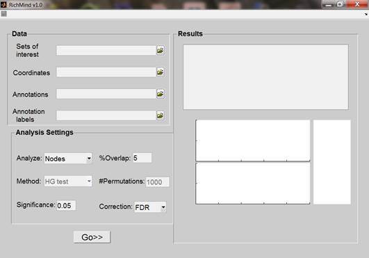
Input:

The following parameters should be provided for execution:

Sets of interest: full path of the file containing all sets of positions/position pairs of interest. For position groups, the file can be (1) a tabular text (.txt) in which each line contains a numerical node identifier followed by a numerical group identifier, (2) a matlab file (.mat) of a numerical matrix in which each row contains a numerical node identifier followed by a numerical group identifier or (3) one/more 3D fMRI NIfTI files (.nii or .img) in which all voxels assigned to a specific SOI are given a corresponding value. For position pairs (connections) groups, two positions are prescribed per line/row in (1) and (2)

Coordinates: full path of the file containing MNI coordinates of all positions that should be considered for the analysis. This set (called the background set) has a crucial effect on the analysis results and should include all positions used in the initial analysis that yielded the interest groups. The file can be (1) a tabular text (.txt) in which each line contains the MNI coordinates of a single position, or (2) a matlab file (.mat) of a numerical matrix in which each row contains the MNI coordinates of a single position.

Annotations: full path of the file containing a numerical annotation for each position in the background set. The file can be (1) a NIfTI image file (.nii or .img) or (2) a tabular text file (.txt) in which each line contains the index of a position followed by a numerical annotation. The index of a position is determined by its ordinal number in the coordinates file

Recall that the annotation is mapping of each neural position to a corresponding term (or terms), such as anatomic labels, known functions, pathology association etc. The annotation defines the terms that are tested for enrichment. For position groups, each annotation represented in a group is tested for enrichment, whereas in the case of connection groups, each connection is assigned with a “paired annotation” according to the annotations of the positions it connects. All paired annotations represented in the groups are then tested for enrichment.

Annotation labels: (optional) full path of a tab delimited text (.txt) file containing a textual label for each numerical annotation given in the node annotation file. Each line contains a numerical annotation followed by the label of the term corresponding to it.

Sample data sets are provided with the software.

Analysis settings:

Method: enrichment calculation method (default is HG-test). When analyzing connection sets, this parameter can be set to Connection permutations (i.e. degree preserving permutations; DPP, which simulate random graphs with a fixed degree sequences) or Label permutations (permuting annotations while preserving their size).

To simulate random graphs with fixed degree sequences, we use a heuristic edge rewiring algorithm (Maslov and Sneppen, 2002; Maslov et al., 2004). Starting from the initial graph G, a pair of edges (uv, wx) such that all of ux,uw,wu,wv are non-edges is randomly chosen, and changed with equal probabilities to (ux, wv) or (uw, vx). This rewiring is performed QM times, with Q = 100, leading to a uniform sampling of Ω (Milo et al., 2003; Pradines et al., 2005).

#Permutations: the required number of permutations in case the selected method I permutation-based (default is 1000). Possible range: 100-500000.

Significance: p-value threshold for each test (default is 0.05)

Correction: Multiple testing correction approach (Bonferroni/FDR/None)

Overlap: The minimum number of elements annotated by a term within a group that is required in order to test for enrichment. This parameter can be used to prevent testing enrichment for terms scarcely represented within a group (default is 5).

Analyzed elements: specifies whether the analysis is conducted on nodes or connections.

Output:

After analysis the following output is presented

Textual report: A table containing, for each identified enrichment, the following information: group ID, enriched annotation term, corrected p-value, representation size (number of elements in the set that are annotated by the term) and frequency ratio (i.e. the ratio between the frequency of annotation representation within group and the frequency of its representation in the background set).

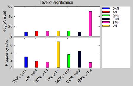
Frequency ratio bar chart: a bar plot (bottom plot in the figure below) displaying, for each enrichment result, its frequency ratio. Bars are colored according to enriched terms (single color for node enrichment and two colors for connection enrichment).

P-value bar chart: a bar plot (top plot in the figure below) displaying, for each enrichment result, the –log(p-value) of that enrichment. Bars are colored according to the enriched terms.

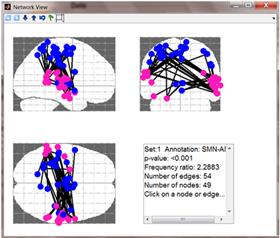
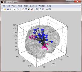
2 and 3D Network view: Upon clicking on one of the lines in the textual report, a 2D – 3 cuts network view is displayed in a separate window (see left-hand figure below). It shows all nodes/connections that are common between the analyzed group and the enriched term (i.e. the nodes/connections that generate the enrichment result). Nodes are colored according to their annotations. Upon pressing the 3D tool-button () in the 2D network view, a corresponding 3D view is displayed (see right-hand figure below).

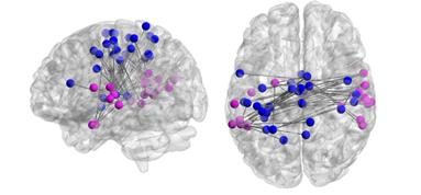
Output export: all outputs can be exported to text and images: text reports and a Matlab structure which contains all results can be exported by clicking on the save tool button located in the top left corner of the main window. A 2D network view can be exported to image file formats or saved as a matlab figure using the save tool-button located in the tool bar of the 2D network window. In addition, input files for BrainNet 3D visualization tool (Xia et al., 2013) can be generated and exported for by pressing the BrainNet tool-button () located in the tool bar of the corresponding 2D network window. A display generated by loading these files to the BrainNet software is shown in the figure below.

References:

Maslov, S. & Sneppen, K. (2002) 'Specificity and stability in topology of protein networks', Science, 296(5569), pp. 910-913.

Maslov, S., Sneppen, K. & Zaliznyak, A. (2004) 'Detection of topological patterns in complex networks: correlation profile of the internet', Physica A: Statistical Mechanics and its Applications, 333, pp. 529-540.

Milo, R., Kashtan, N., Itzkovitz, S., Newman, M. E. & Alon, U. (2003) 'Uniform generation of random graphs with arbitrary degree sequences', arXiv preprint cond-mat/0312028, 106, pp. 1-4.

Pradines, J. R., Farutin, V., Rowley, S. & Dancík, V. (2005) 'Analyzing protein lists with large networks: edge-count probabilities in random graphs with given expected degrees', Journal of Computational Biology, 12(2), pp. 113-128.

Xia, M., Wang, J. & He, Y. (2013) 'BrainNet Viewer: a network visualization tool for human brain connectomics', PLoS One, 8(7), p. e68910.